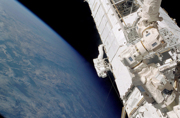
Piers Sellers during a spacewalk outside of the International Space Station. Credit: NASA
Astronaut and scientist Piers Sellers is no longer with us, but his words still resonate.
A posthumous plea from Sellers arrived in July 2018 in the form of an article in PNAS. The topic was one that he cared deeply about: building a better space-based system for observing and understanding the carbon cycle and its climate feedbacks.
As NASA’s Patrick Lynch reported, Sellers wrote the paper along with colleagues at NASA’s Jet Propulsion Laboratory and the University of Oklahoma. Work on the paper began in 2015, and Sellers continued working with his collaborators up until about six weeks before he died. They carried on the research and writing of the paper until its publication in July 2018.
The carbon cycle refers to the constant flow of carbon between rocks, water, the atmosphere, plants, soil, and fossil fuels. Climate change feedbacks—natural effects that may amplify or diminish the human emissions of greenhouse gases—are one of the most poorly understood aspects of climate science.
Here is how Sellers and colleagues characterized the current state of the carbon cycle in the PNAS article:
“It is quite remarkable and telling that human activity has significantly altered carbon cycling at the planetary scale. The atmospheric concentrations of carbon dioxide (CO2) and methane (CH4) have dramatically exceeded their envelope of the last several million years.”

They also explain in detail how we have altered the carbon cycle:
“The perturbation by humans occurs first and foremost through the transfer of carbon from geological reservoirs (fossil fuels) into the active land–atmosphere–ocean system and, secondarily, through the transfer of biotic carbon from forests, soils, and other terrestrial storage pools (e.g., industrial timber) into the atmosphere.”
Scientists understand the broad outlines of how this works relatively well. What worried Sellers was the potential curve balls the climate might throw at us with unanticipated feedbacks. They addressed some of the the challenges in understanding how climate change might affect concentrations of carbon dioxide and methane through feedbacks.
For carbon dioxide:
“While experimental studies consistently show increases in plant growth rates under elevated CO2 (termed carbon dioxide fertilization), the extrapolation of even the largest-scale experiments to ecosystem carbon storage is problematic, and some ecologists have argued that the physiological response could be eliminated entirely by restrictions due to limitation by nutrients or micronutrients. However, there is recent evidence from the atmosphere that suggests increasing CO2 enhances terrestrial carbon storage, leading to the continued increase in land uptake paralleling CO2 concentrations.”
As we detailed in a separate story, the situation is even more complicated for methane. Sellers and his colleagues explained some of the challenges in understanding the feedbacks that affect that potent greenhouse gas this way:
“Atmospheric methane is currently at three times its preindustrial levels, which is clearly driven by anthropogenic emissions, but equally clearly, some of the change is because of carbon-cycle–climate feedbacks. Atmospheric CH4 rose by about 1 percent per year in the 1970s and 1980s, plateaued in the 1990s, and resumed a steady rise after 2006. Why did the plateau occur? These trends in atmospheric methane concentration are not understood. They may be due to changes in climate: increases in temperature, shifts in the precipitation patterns, changes to wetlands, or proliferation in the carbon availability to methane-producing bacteria.”
The consequences of the gaps in understanding could be significant.
“Terrestrial tropical ecosystem feedbacks from the El Nino drove an ∼2-PgC increase in global CO2 emissions in 2015. If emissions excursions such as this become more frequent or persistent in the future, agreed-upon mitigation commitments could become ineffective in meeting climate stabilization targets. Earth system models disagree wildly about the magnitude and frequency of carbon–climate feedback events, and data to this point have been astonishingly ineffective at reducing this uncertainty.”
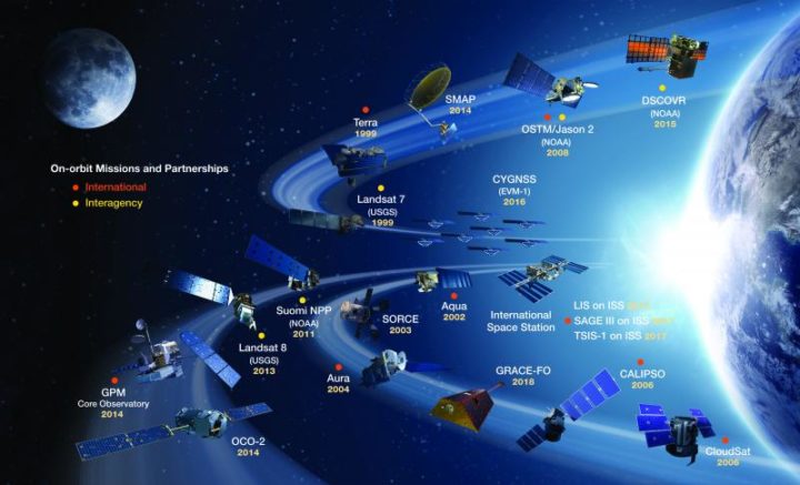
NASA’s current missions and partnership missions in orbit. Credit: NASA
Sellers and his colleagues do offer a solution. It has much to do with satellites.
“Space-based observations provide the global coverage, spatial and temporal sampling, and suite of carbon cycle observations required to resolve net carbon fluxes into their component fluxes (photosynthesis, respiration, and biomass burning). These space-based data substantially reduce ambiguity about what is happening in the present and enable us to falsify models more effectively than previous datasets could, leading to more informed projections.”
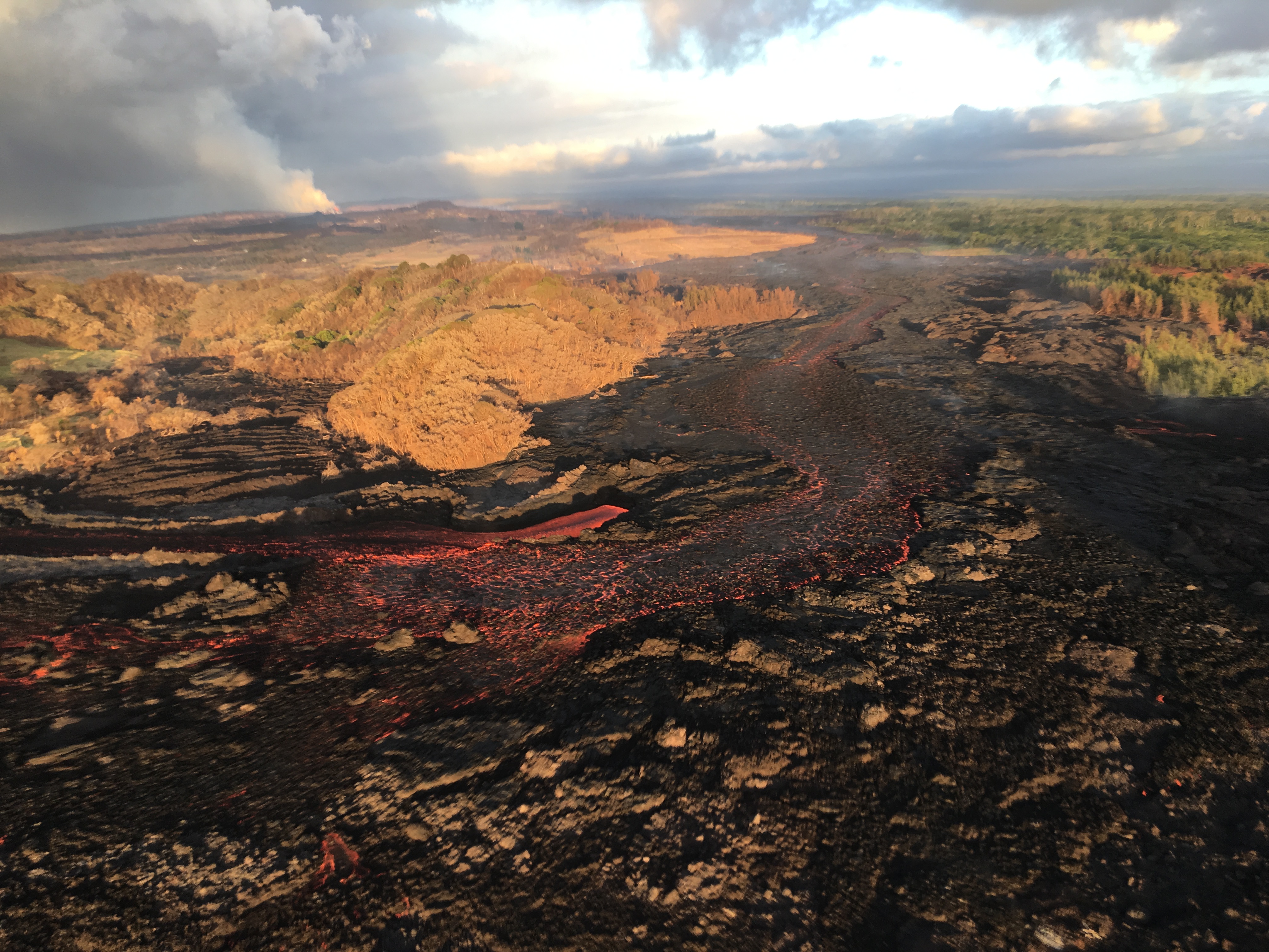
For more than two months, lava has been pouring from part of Hawaii’s Kilauea volcano, destroying homes and remaking the land surface. More data and imagery of the eruption is flowing in from satellites, drones, and ground-based sensors than Earth Observatory can cover, but here are a few striking images that we would be remiss not to share.
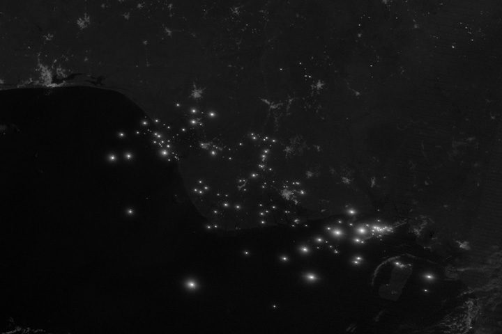
By The Lava’s Early Light 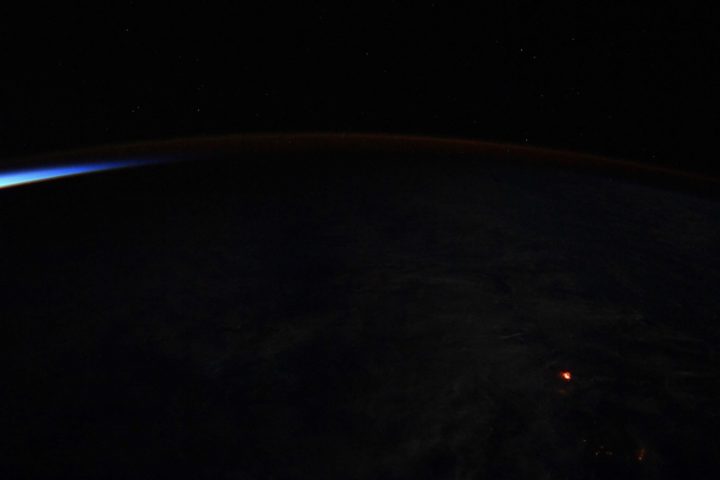
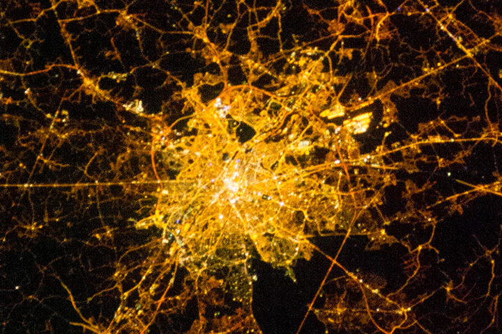
NASA Astronaut Ricky Arnold tweeted this nighttime photograph of lava on June 20, 2018. If the Star Spangled Banner had been composed in Hawaii rather than Baltimore, maybe “lava’s early light” would have made it into the lyrics. Credit: NASA
The Wrong Side of the Lava Flow
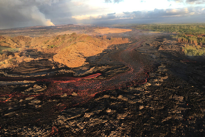
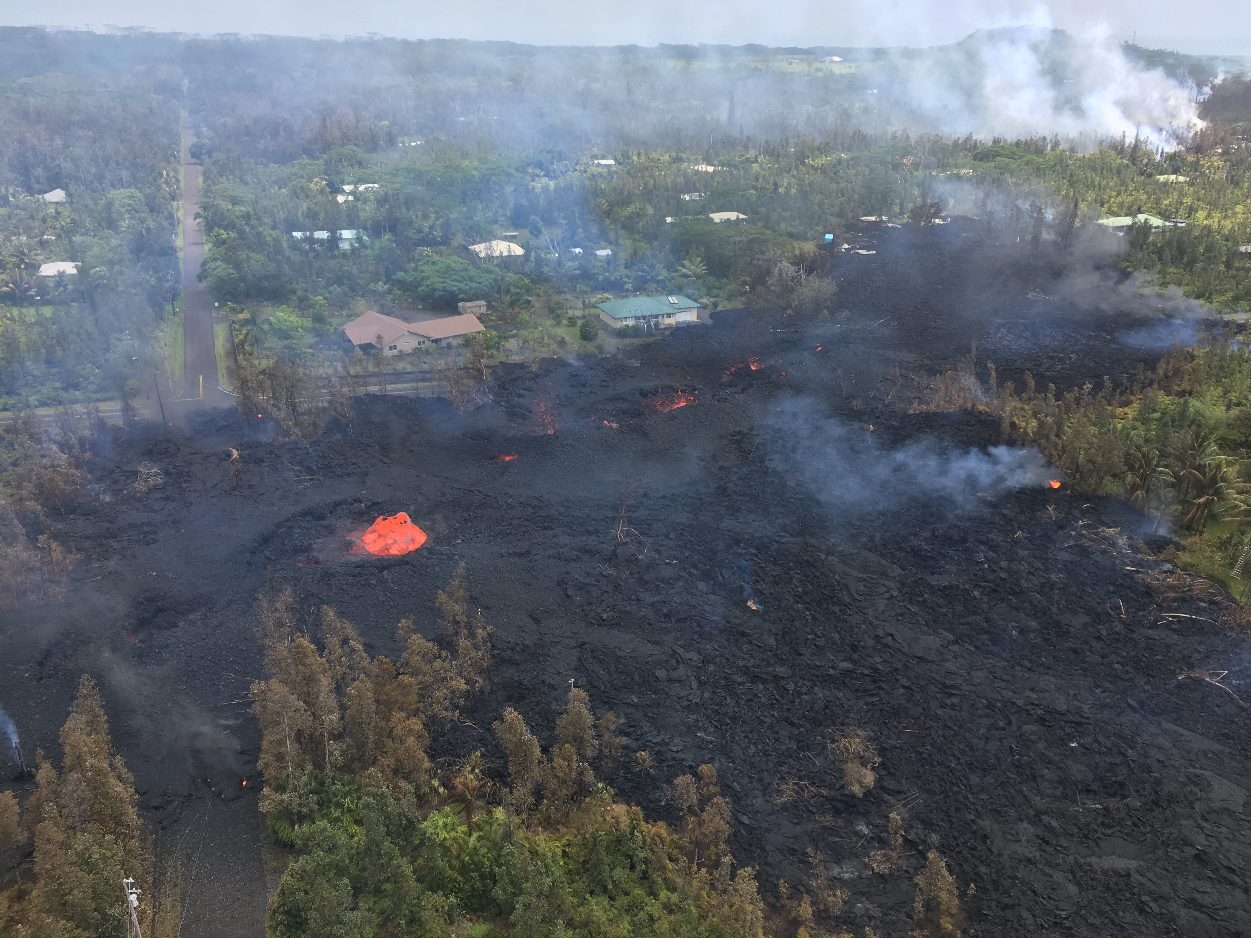
Notice the stark differences in landscapes on the northern and southern sides of the lava channel. With trade winds blowing heat and volcanic gases to the southwest, the north side remained green. Vegetation on the south side, yellowed and brown, took a battering. This aerial photograph was taken on July 10, 2018. Image Credit: USGS.
A Colorful Satellite Perspective on a Collapsing Caldera
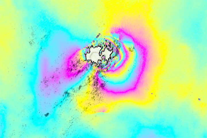
As lava flows from some parts of Kilauea, other parts of the volcano have been sinking. In the case of the summit caldera, the rate of subsidence has been dramatic. This interferometric synthetic aperature radar (InSAR) image, or interferogram, shows surface movement at the summit caldera between June 9 and June 23. Each cycle of yellow-blue-purple indicates approximately 5 inches (13 centimeters) of movement. Areas where the colorful lines are the closest have shifted the most. The data was collected by Advanced Land Observing Satellite-2 (ALOS-2), a Japanese Aerospace Exploration Agency (JAXA) mission. Read more about this image and type of data from NASA’s Disasters Program. Image Credit: NASA/JAXA.
The Same Caldera Collapse Seen from the Ground
This sequence of images shows rapid subsidence of the caldera floor, along with the development of scarps. One photograph is shown per day between June 13 and 24. The photos were taken from the southern caldera rim, near Keanakāko‘i Crater, and face north. Image Credit: USGS.
Laze Billows into the Air as Lava Pours into the Sea
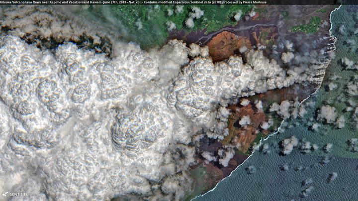
In this Sentinel-2 image, a large plume of laze—steam, volcanic gases, and shards of glass—blows west over Hawaii as lava poured into the sea on June 27, 2018. Pierre Markuse created this image using data from Sentinel-2, a satellite managed by the European Space Agency. He regularly downloads and processes Sentinel and Landsat satellite data and has posted dozens of Kilauea images on Flickr. Image Credit: ESA/Sentinel-2/Markuse
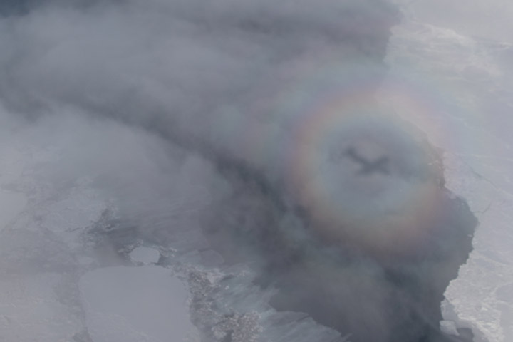
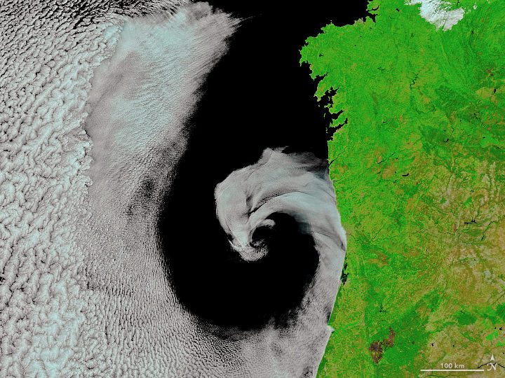
Earlier this month, we showed a space-based view of a glory—a colorful, circular optical phenomenon caused by water droplets scattering light. The Moderate Resolution Imaging Spectroradiometer on the Terra and Aqua satellites can see only a cross section of the glory, making it appear in satellite imagery as two elongated bands parallel to the path of the satellite.
To the Earth-bound observer, however, glories take on a circular shape. You might have seen one while on an aircraft. From this perspective, passengers on the side of the plane directly opposite the Sun can sometimes see the plane’s shadow on the clouds below. This position is also where glories can be observed as the cloud’s water droplets scatter sunlight back toward a source of light.
Before aviation, the phenomenon was often seen by mountain climbers; the glory encircling the climber’s shadow on the clouds below. Today, pilots and passengers have a good chance of seeing them, earning the phenomenon the name “glory of the pilot” or “pilot’s halo.”
But you still have to be flying close enough to the cloud deck for the phenomenon to be visible, which is one of the reasons why they are frequently spotted by scientists and crew with NASA’s Operation IceBridge mission. The mission makes annual flights over Earth’s poles to map the ice; flights are relatively low, long, and frequent. Glories are not part of the mission’s science goals—in fact, clouds can interfere with the collection of science data. But they are on the list of natural wonders that IceBridge scientists witness in the field.
Jeremy Harbeck, a sea ice scientist at NASA’s Goddard Space Flight Center, snapped the top photograph of a glory on April 18, 2018, during an IceBridge science flight over the Chukchi Sea. (See the full image and other photographs shot by Harbeck during the Arctic 2018 IceBridge campaign here.)
“I remember having taken more images of glories, especially down over Antarctica, as we see them quite often down there,” Harbeck said. “From what I remember, they’re not outside the window all the time, but you can catch them here and there on flights when conditions are right.”
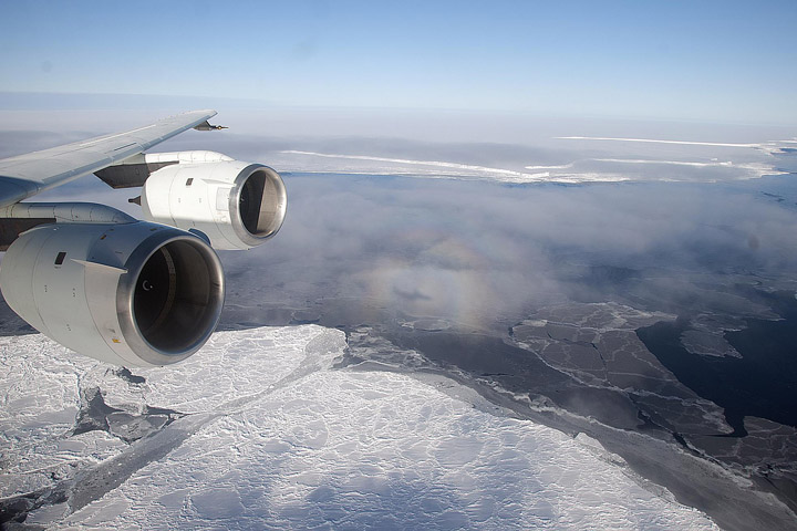
One such Antarctic glory is visible in the image above, snapped by Michael Studinger during an IceBridge flight on October 26, 2010. Read more about that image here.

Orbit Pavilion. Image courtesy of NASA/Jet Propulsion Laboratory-Caltech/The Studio/Dan Goods
Sure, space may be silent, or at least absent the sound waves that human ears can hear. But put that aside for a moment, and try to imagine the sound of a satellite orbiting hundreds of miles above Earth’s surface.
Now imagine 19 sounds for 19 Earth-observing satellites — the murmur of ocean waves for a spacecraft that studies the oceans, or the howl of winds for one that studies hurricanes. Then swirl all of those sounds into a shell-shaped silver sculpture that looks like something from a sci-fi film.
Put the shell at the Huntington Library in southern California, walk inside, and you have Orbit Pavilion — an immersive piece of art and science communication designed to envelop people in sounds that represents the orbital movements of NASA’s fleet of Earth-observing satellites.
Dan Goods and David Delgado, artists working at The Studio at NASA Jet Propulsion Laboratory, initially developed the sound concept. They commissioned sound artist Shane Myrbeck to compose the soundscape, and Jason Klimoski and Lesley Chang of StudioKCA to envision and design a form.
Myrbeck describes the pavilion’s soundscape this way:
“The piece is in two parts, each with one sound following the path of a satellite. One section demonstrates the movement of the satellites by compressing a day’s worth of trajectory data into one minute, so listeners are enveloped by a symphony of 19 sounds swirling around them. The other section represents the real-time position of the spacecraft: each satellite currently in our hemisphere will “speak” in sequence, and when a sound is playing, if a listener points to the direction of the sound, they are pointing to the satellite orbiting hundreds of miles above us….These satellites are all part of Earth science missions, studying our atmosphere, oceans, and geology — they are helping us better understand how our planet is changing, and potentially how we can be better stewards of it. In that way I see them as kind of sentinels or protectors.”
The result, as Myrebeck had hoped, is both enveloping and comforting.

Information about the orbits of 17 satellites and two sensors on the International Space Station feed into the Orbit Pavilion. Image Credit: StudioKCA

The current fleet of Earth-observing satellites. Image Credit: NASA/EOSPSO
For a deeper dive into the diversity of the data these satellites collect, try searching a satellite’s name on Visible Earth. Or browse NASA Earth Observatory’s global maps sections and Image of the Day archive.
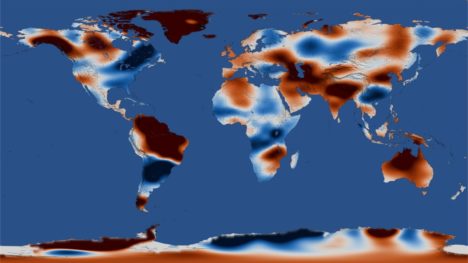
For instance, the map below helped me understand our planet a little bit better. It depicts more than a decade of cloudiness data as observed by the MODIS sensor. Blue shows areas where clouds were infrequent; white indicates areas where they were common.

Image Credit: NASA Earth Observatory, based on data from MODIS.
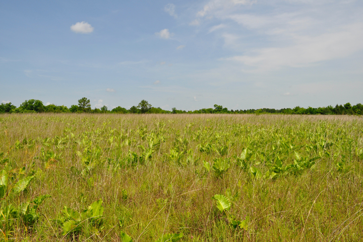
Photo by JoVonn Hill, Mississippi State University.

NASA Earth Observatory images by Joshua Stevens.
This month we published a satellite image and map of the southern United States featuring the Black Belt Prairie—a crescent-shaped swath of land running through Mississippi and Alabama named for its characteristically dark, fertile soil. Most of the fertile soils are cultivated, contrasting sharply with adjacent forested areas.
Grassland expert JoVonn Hill of Mississippi State University noted that in the 1830s, the Black Belt contained about 356,000 acres of prairie. Today, less than 1 percent of prairie land remains. One such prairie remnant is the Pulliam Prairie in Chickasaw County, Mississippi. Hill snapped this photograph (top image) of native grassland within the Pulliam Prairie, which in total spans about 250 acres. That’s a decent size for Black Belt prairie remnants, most of which span just 5-20 acres.
Pulliam Prairie is one of the most significant prairie remnants in Mississippi, given its large area and the diversity of species found there. Black Belt prairie remnants dot the landscape in Alabama too, all of which are important sites for the supporting an array of native vegetation and habitat. As Hill noted in our initial story about the region: “Find a remnant of the Black Belt prairie, and you could see some of its unique grassland birds; more than 200 species of plants, 1,000 species of moths, 107 species of bees, 33 species of grasshoppers, and 53 species of ants.”

The Telstar satellite (left) and the 1974 Telstar Durlast, the official ball of the 1974 World Cup. Image Credit: Bell Labs/Shine 2010
Goooooooal!!!! The 2018 FIFA World Cup kicked off on June 14, 2018.
Here’s a bit of Cup trivia you may not know. In 1962, NASA launched a small, spherical communications satellite called Telstar that ended up altering the look of the balls used in the World Cup.
Telstar was the first active communications satellite and the first commercial payload in space. By sending television signals, telephone calls, and fax images from space, the 3-foot-long satellite kicked off a whole new era in telecommunications—and soccer ball design.
There’s a direct line between the distinctive black and white patterning of Telstar’s hull and solar panels and the Adidas ball used as the official ball of the 1970 World Cup in Mexico and the 1974 World Cup in West Germany. While earlier generations of soccer balls were brown and did not show up well on television, the 1970 and 1974 balls featured the now iconic 32-panel design of alternating white hexagons and black pentagons, a pattern that closely resembled Telstar. Fittingly, that first ball was called Telstar Elast; the official ball in 2018, a nod to the 1970 ball, is called the Telstar 18.
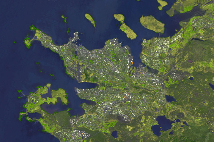
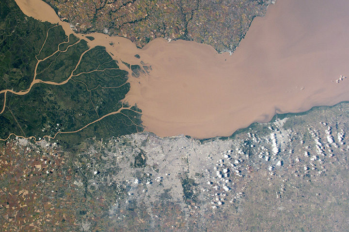
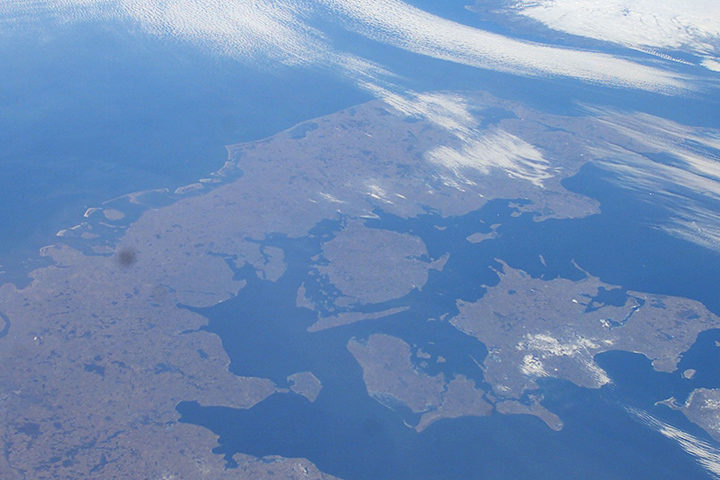
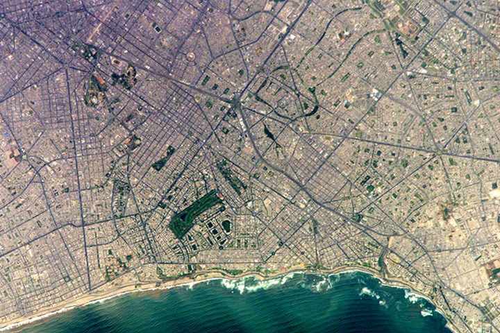
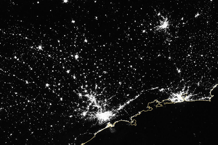
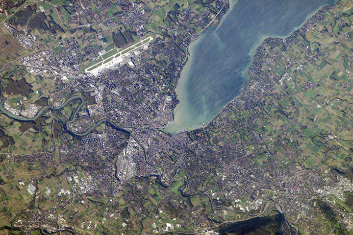
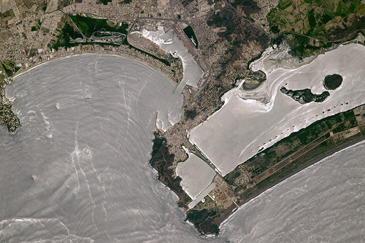
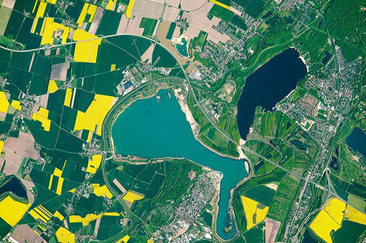
To celebrate the World Cup, Earth Observatory is planning to dig into its archives. For key games, we’ll grab one image for each of the two countries going head to head. Can you guess which image goes with which country? Just click on the images below to find out. Enjoy the tournament!
June 14:
Russia 5 — 0 Saudi Arabia
June 15
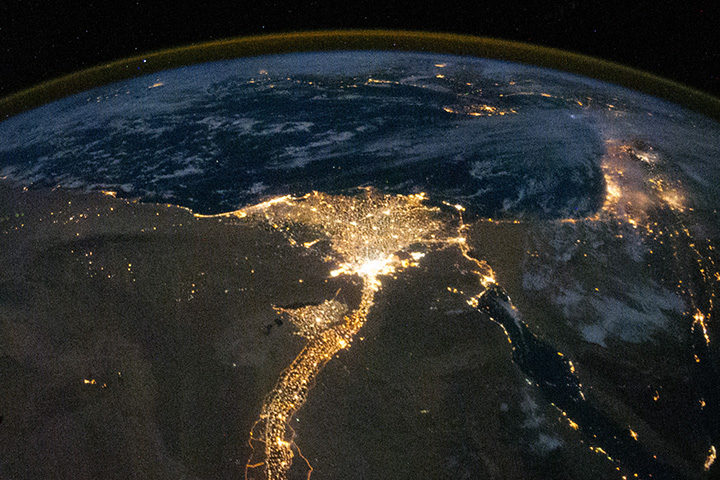
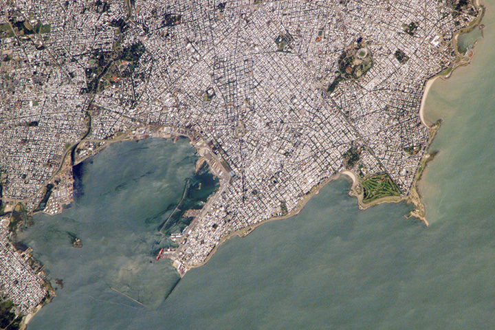
Uruguay 1 — 0 Egypt
Iran 1 — 0 Morocco
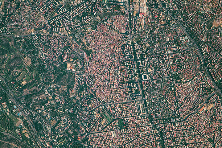
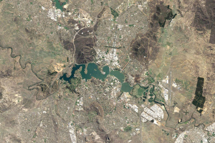
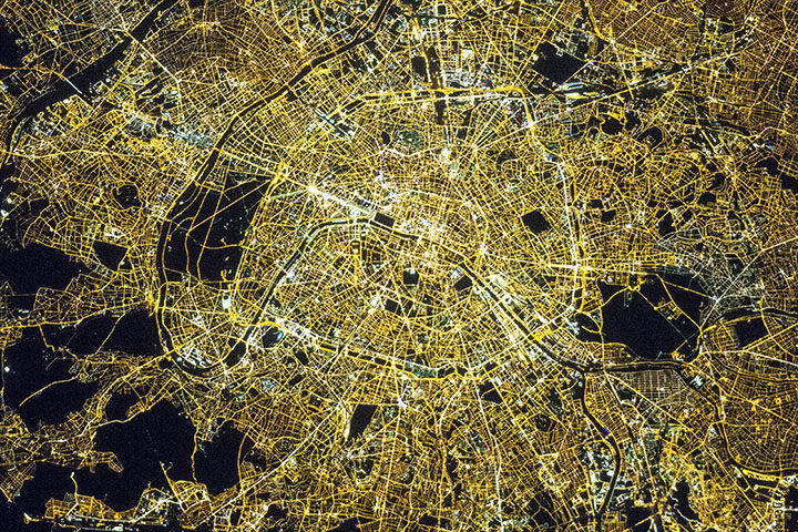
Portugal 3 — 3 Spain
June 16
France 2 — 1 Australia
Iceland 1 — 1 Argentina
Peru 0 — 1 Denmark
Croatia 2 — 0 Nigeria
June 17
Costa Rica 0 — 1 Serbia
Brazil 1 — 1 Switzerland
Mexico 1 — 0 Germany
June 18
Sweden vs. Korea Republic
Belgium vs. Panama
Tunisia vs. England

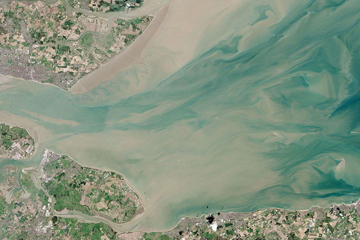
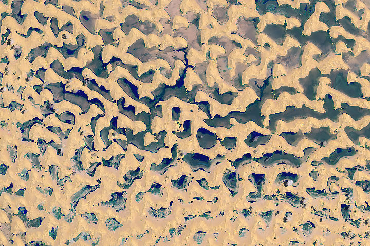
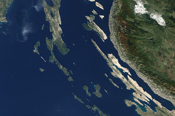
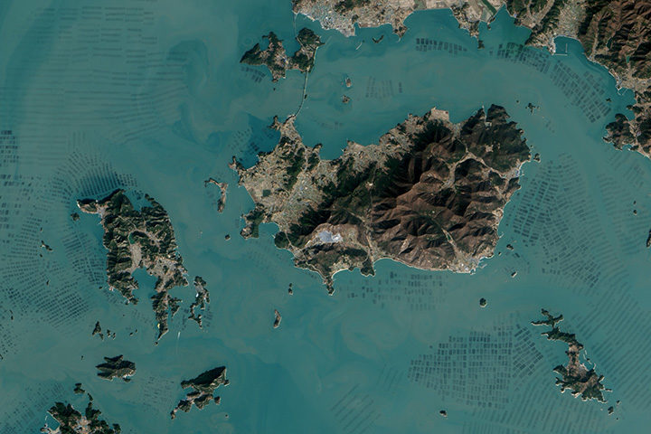
Every month on Earth Matters, we offer a puzzling satellite image. The June 2018 puzzler is above. Your challenge is to use the comments section to tell us what we are looking at and why this place is interesting.
How to answer. You can use a few words or several paragraphs. You might simply tell us the location. Or you can dig deeper and explain what satellite and instrument produced the image, what spectral bands were used to create it, or what is compelling about some obscure feature in the image. If you think something is interesting or noteworthy, tell us about it.
The prize. We can’t offer prize money or a trip to Mars, but we can promise you credit and glory. Well, maybe just credit. Roughly one week after a puzzler image appears on this blog, we will post an annotated and captioned version as our Image of the Day. After we post the answer, we will acknowledge the first person to correctly identify the image at the bottom of this blog post. We also may recognize readers who offer the most interesting tidbits of information about the geological, meteorological, or human processes that have shaped the landscape. Please include your preferred name or alias with your comment. If you work for or attend an institution that you would like to recognize, please mention that as well.
Recent winners. If you’ve won the puzzler in the past few months or if you work in geospatial imaging, please hold your answer for at least a day to give less experienced readers a chance to play.
Releasing Comments. Savvy readers have solved some puzzlers after a few minutes. To give more people a chance to play, we may wait between 24 to 48 hours before posting comments.
Good luck!
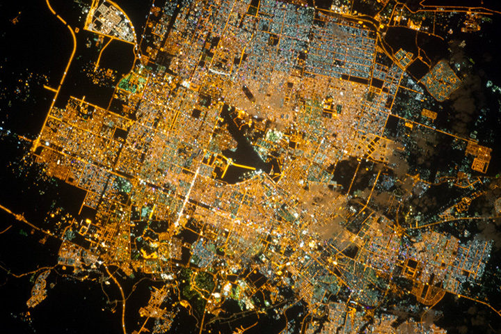
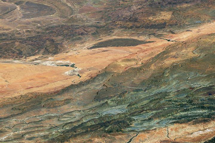
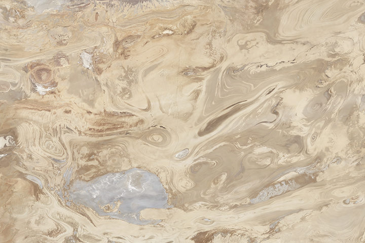
Answer: The Rub’ al-Khali is the world’s largest contiguous sand desert, located on the Arabian Peninsula. It is typically one of the driest places on Earth. The image above shows the desert after rainwater associated with Tropical Cyclone Mekuno pooled between the dunes. Congratulations to John Morales for being the first to correctly name the desert, and to AIYED for also naming the storm system. Read more about the image in our June 16, 2018, Image of the Day.
This is a cross-post of a story by Ellen Gray. It provides deeper insight into our May 23 Image of the Day.
Six months after GRACE launched in March 2002, we got our first look at the data fields. They had these big vertical, pole-to-pole stripes that obscured everything. We’re like, holy cow this is garbage. All this work and it’s going to be useless.
But it didn’t take the science team long to realize that they could use some pretty common data filters to remove the noise, and after that they were able to clean up the fields and we could see quite a bit more of the signal. We definitely breathed a sigh of relief. Steadily over the course of the mission, the science team became better and better at processing the data, removing errors, and some of the features came into focus. Then it became clear that we could do useful things with it.
It only took a couple of years. By 2004, 2005, the science team working on mass changes in the Arctic and Antarctic could see the ice sheet depletion of Greenland and Antarctica. We’d never been able before to get the total mass change of ice being lost. It was always the elevation changes – there’s this much ice, we guess – but this was like wow, this is the real number.
Not long after that we started to see, maybe, that there were some trends on the land, although it’s a little harder on the land because with terrestrial water storage — the groundwater, soil moisture, snow, and everything. There’s inter-annual variability, so if you go from a drought one year to wet a couple years later, it will look like you’re gaining all this water, but really, it’s just natural variability.
By around 2006, there was a pretty clear trend over Northern India. At the GRACE science team meeting, it turned out another group had noticed that as well. We were friendly with them, so we decided to work on it separately. Our research ended up being published in 2009, a couple years after the trends had started to become apparent. By the time we looked at India, we knew that there were other trends around the world. Slowly not just our team but all sorts of teams, all different scientists around the world, were looking at different apparent trends and diagnosing them and trying to decide if they were real and what was causing them.
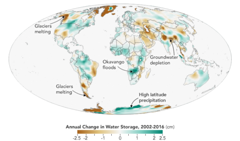
I think the map, the global trends map, is the key. By 2010 we were getting the broad-brush outline, and I wanted to tell a story about what is happening in that map. For me the easiest way was to just look at the data around the continents and talk about the major blobs of red or blue that you see and explain each one of them and not worry about what country it’s in or placing it in a climate region or whatever. We can just draw an outline around these big blobs. Water is being gained or lost. The possible explanations are not that difficult to understand. It’s just trying to figure out which one is right.
Not everywhere you see as red or blue on the map is a real trend. It could be natural variability in part of the cycle where freshwater is increasing or decreasing. But some of the blobs were real trends. If it’s lined up in a place where we know that there’s a lot of agriculture, that they’re using a lot of water for irrigation, there’s a good chance it’s a decreasing trend that’s caused by human-induced groundwater depletion.
And then, there’s the question: are any of the changes related to climate change? There have been predictions of precipitation changes, that they’re going to get more precipitation in the high latitudes and more precipitation as rain as opposed to snow. Sometimes people say that the wet get wetter and the dry get dryer. That’s not always the case, but we’ve been looking for that sort of thing. These are large-scale features that are observed by a relatively new satellite system and we’re lucky enough to be some of the first to try and explain them.
The past couple years when I’d been working the most intensely on the map, the best parts of my time in the office were when I was working on it. Because I’m a lab chief, I spend about half my time on managerial and administrative things. But I love being able to do the science, and in particular this, looking at the GRACE data, trying to diagnose what’s happening, has been very enjoyable and fulfilling. We’ve been scrutinizing this map going on eight, nine years now, and I really do have a strong connection to it.
What kept me up at night was finding the right explanations and the evidence to support our hypotheses – or evidence to say that this hypothesis is wrong and we need to consider something else. In some cases, you have a strong feeling you know what’s happening but there’s no published paper or data that supports it. Or maybe there is anecdotal evidence or a map that corroborates what you think but is not enough to quantify it. So being able to come up with defendable explanations is what kept me up at night. I knew the reviewers, rightly, couldn’t let us just go and be completely speculative. We have to back up everything we say.
The world is a complicated place. I think it helped, in the end, that we categorized these changes as natural variability or as a direct human impact or a climate change related impact. But then there can be a mix of those – any of those three can be combined, and when they’re combined, that’s when it’s more difficult to disentangle them and say this one is dominant or whatever. It’s often not obvious. Because these are moving parts and particularly with the natural variability, you know it’s going to take another 15 years, probably the length of the GRACE Follow-On mission, before we become completely confident about some of these. So it’ll be interesting to return to this in 15 years and see which ones we got right and which ones we got wrong.
You can read about Matt’s research here: https://go.nasa.gov/2L7LXoP.
An active fissure in Leilani Estates subdivision. This photo shows fissure 7 on May 5, 2018. Image Credit: U.S. Geological Survey
You have probably seen dramatic images and videos of several new fissure eruptions cracking open the land surface in Hawaii, emitting plumes of gas, and spitting up fountains of lava in the middle of a residential neighborhood.
If you are tracking Kilauea’s eruptions, the U.S. Geological Survey Hawaiian Volcano Observatory (HVO) and Hawaii County Civil Defense are the best sources for the latest information. HVO releases status reports, photos, videos, maps, and near-real time data that are invaluable to understanding what is happening. Hawaii County issues frequent alerts with details about evacuations, road closures, and the status of utilities.
If you want to dig into the science of this eruption, HVO and the Smithsonian Global Volcanism Program both have informative summaries that synthesize what scientists know of Kilauea’s geologic history. There are also knowledgeable volcanologists tracking the eruption closely and offering science-based commentary. Janine Krippner of Concord University (@janinekrippner) is a trained volcanologist who tweets regularly about developments. Ken Rubin @kenhrubin), based at the University of Hawaii, does the same. Erik Klemetti, a volcanologist at Denison University, is reporting on the eruption on his Rocky Planet blog.
To extend the scientific conversation, Earth Matters reached out to a handful of researchers from NASA and elsewhere who are monitoring the volcano. Among those who responded were Simon Carn (Michigan Technological University), Ashley Davies (NASA Jet Propulsion Laboratory), Jean-Paul Vernier (NASA Langley Research Center), Verity Flower (Universities Space Research Association/NASA Goddard Space Flight Center) and Krippner.
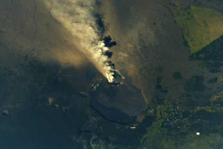
NASA astronaut Drew Feustel tweeted this photograph of a volcanic plume at the summit of Kilauea on May 13, 2018. Image Credit: NASA
Can you briefly describe the steps that happen in an eruption like we’re seeing with Kīlauea?
“First, USGS HVO tiltmeters recorded inflation of the volcano. This was caused by magma moving up from depth, causing the volcano to bulge outwards. The lava lake level in the summit caldera (Halema’uma’u) rose, an indication of the influx of magma into the volcanic plumbing system. Local seismic activity increased due to rock breaking as magma forces its way upwards, and as the broader volcanic edifice adjusted and reacted to the changing stress field. As magma rose, more volcanic gas (including sulfur dioxide) was released. As magma moved into the near surface East Rift Zone, the summit started to deflate, and the lava lake level dropped. There were structural adjustments along the rift, from the summit, to Pu’u O’o, and along the rift, causing earthquakes. Then lava erupted, the whole system began to depressurize, and deflation continued.”
– Ashley Davies
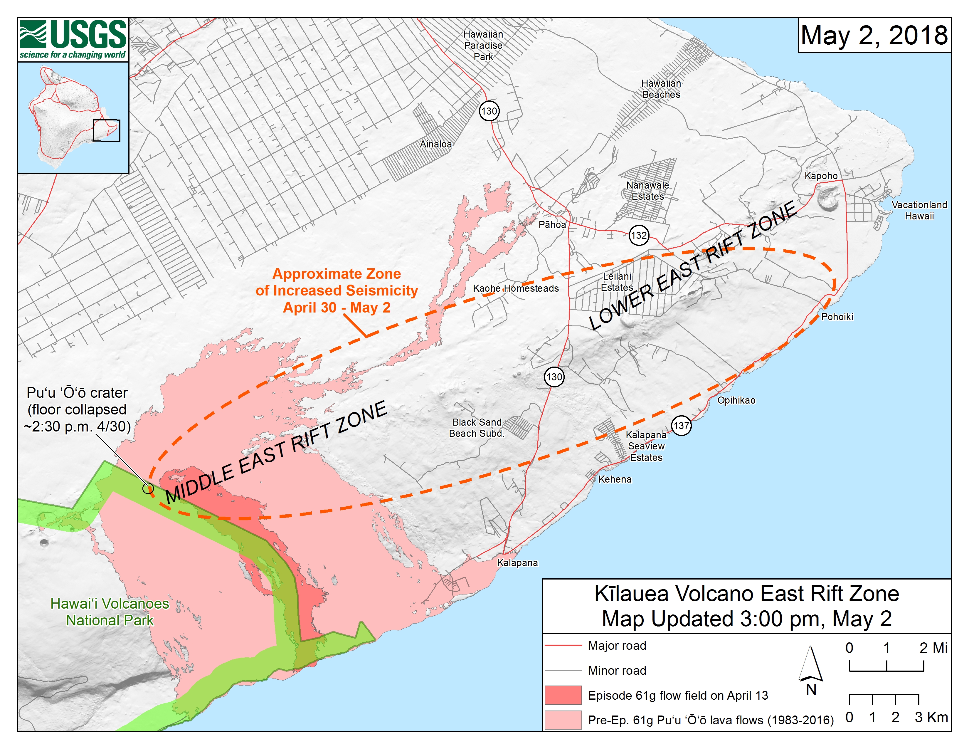
Starting on the afternoon of Monday, April 30, 2018, magma beneath Pu‘u ‘Ō‘ō drained and triggered the collapse of the crater floor. Within hours, earthquakes began migrating east of Pu‘u ‘Ō‘ō, signaling an intrusion of magma along the middle and lower East Rift Zone. Map credit: U.S. Geological Survey. More maps here.
How would you describe the significance or scope of this eruption?
“This eruption is part of the normal life cycle of Kilauea volcano and is comparable to past activity. In fact, 90 percent of the surface of Kilauea is less than 1,000 years old — very young on a geologic time scale. The significance of this eruption is that it is directly occurring in the Leilani community. These people need help and support. Even though we all live with natural hazards, no matter where we are, we don’t often imagine it happening to us.” — Janine Krippner
What can we expect to happen next? Is the fissure eruption likely to persist for a long time?
“It could be a major risk to the Leilani Estates area if the eruption continues. So far, the lava flows have not traveled very far from the eruptive fissure. If this changes or the fissure extends in length, then more property will be destroyed and major roads could be cut.”
— Simon Carn
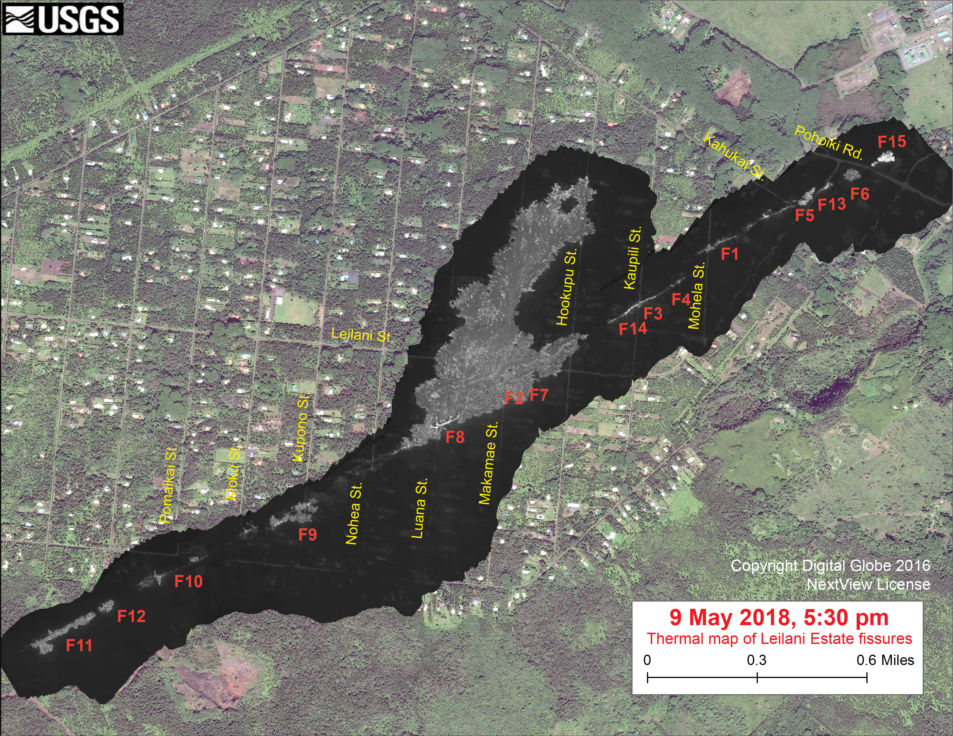
This map overlays a georegistered mosaic of thermal images collected during a U.S. Geological Survey helicopter overflight of the fissures in Leilani Estates on May 9, 2018. The base is a copyrighted satellite image (used with permission) provided by Digital Globe. Temperature in the thermal image is displayed as gray-scale values, with the brightest pixels indicating the hottest areas (white shows active breakouts). Image: Courtesy of USGS, Copyright Digital Globe, NextView License.
“This eruption could persist for quite a while, but it is impossible to tell how long. This is a dynamic situation, and new fissures could start and stop with little to no warning. The risk of lava inundation is real and significant, depending on where lava is extruded at the surface and how much.” — Janine Krippner
Can you address the health hazards associated with sulfur dioxide?
“The problem with sulfur dioxide is that if you breathe it in, it can combine with water in the lungs to create an acid. With sulfur dioxide issuing from the fissures in an inhabited area, it makes for unhealthy concentrations locally. HVO has more on this here.” — Ashley Davies
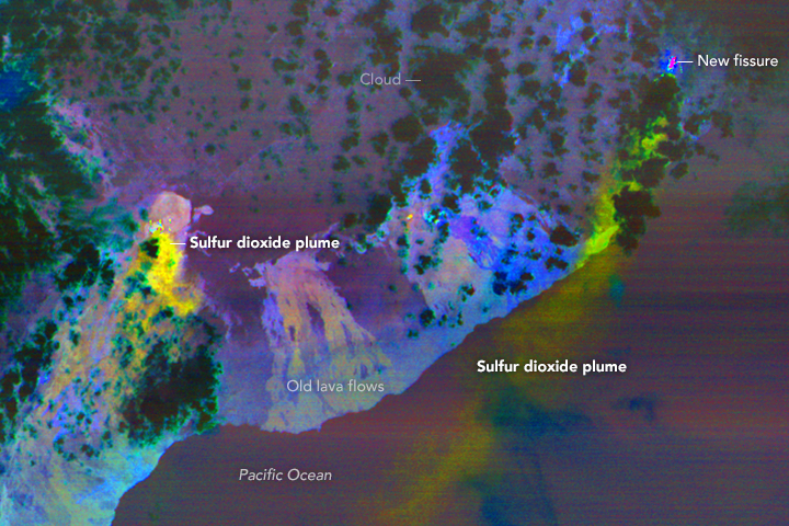
This false-color ASTER image was acquired on May 6, 2018. It shows the sulfur dioxide plume in yellow and yellow-green coming from new activity in Leilani Estates. A smaller, but thicker, sulfur dioxide plume can be seen coming from Kilauea’s main vent. Image Credit: NASA/ASTER
“Sulfur dioxide is a common occurrence in Hawaii, as vog (volcanic smog), which is a mixture of sulfur and aerosols. Sulfur dioxide and/or vog can cause irritation to eyes and airways, causing coughing, wheezing, headaches, and sore throats. People with preexisting conditions, such as asthma, are more at risk. Sulfur dioxide levels have been measured at dangerous and deadly levels near the fissures.” — Janine Krippner
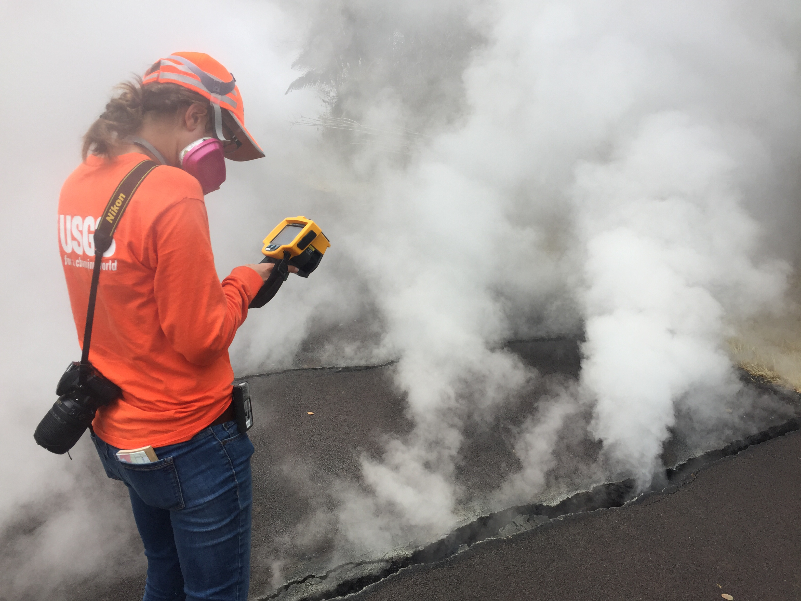
Volcanic gases rise from a fissure on Nohea Street, Leilani Estates. An HVO geologist measured a temperature of 103 degrees C (218 degree F). The asphalt road was describes as “mushy” from the heat. Image Credit: U.S. Geological Survey.
Which satellites sensors are making observations of Kilauea’s plume?
There are several. The Multi-angle Imaging SpectroRadiometer (MISR) can measure the height of plumes from stereo imagery, and makes observations of the size and shape of the particles, which is useful for determining the degree to which the plume is rich in liquid sulfate and water particles versus solid, angular ash particles. The Moderate Resolution Imaging Spectroradiometer (MODIS) and Visible Infrared Imaging Radiometer Suite (VIIRS) are collecting daily snapshots of the amount of particulate matter in the plume — as well as making observations of the sulfur dioxide plumes based on their thermal bands. The Operational Land Imager (OLI) and Advanced Spaceborne Thermal Emission and Reflection Radiometer (ASTER) provide more detailed images, though overpasses are less frequent. Finally, synthetic aperture radar on Sentinel 1 is tracking how much the land deforms as the eruption progresses.
— Verity Flower
To what degree are satellites sensors like OMPS and OMI useful for monitoring sulfur dioxide emissions?
Satellites provide unique information on the total sulfur dioxide mass and spatial distribution in a plume ‘snapshot’, but provide minimal information on sulfur dioxide at ground level. Other techniques provide more localized measurements but can detect surface concentrations. — Simon Carn
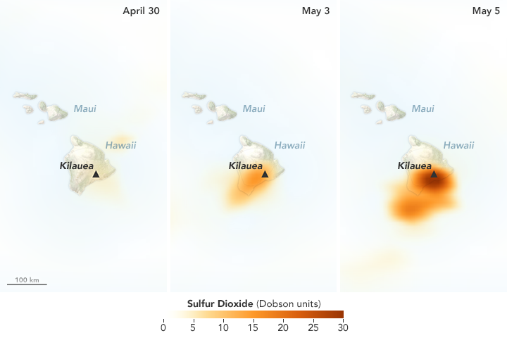
The Ozone Mapping Profiler Suite (OMPS) detected increasing concentrations of sulfur dioxide over Hawaii in May 2018. Image Credit: NASA Earth Observatory. Learn more about this map.
Are there other reasons to monitor volcanic plumes aside from health hazards?
The particles in volcanic ash have sharp, angular edges that can abrade aircraft windows hindering the pilots ability to navigate. Where these ash particles enter aircraft engines the high temperatures cause ash to melt, coating the rotors, air intakes and casings that can lead to engine failure. Plumes can also have effects—sometimes even positive effects—on the wider environment. Ash falls can destroy crops and damage infrastructure during an eruption, but they can also add nutrients to the ocean that fuel phytoplankton blooms and nutrients to the soil that make farmland more fertile on longer timescales. — Verity Flower
Can you tell me anything about the wind patterns around Hawaii?
So far, northwesterly trade winds, which are common in this area, have kept the plume over the ocean. The winds do occasionally shift for short periods, which could bring more volcanic pollution over populated areas. — Verity Flower
What has NASA been doing in response to the eruption?
“The NASA Disasters Program is working with several teams to assess the eruption and make information available to first responders and others. We are working with several instrument teams to monitor the sulfur dioxide plume. We are also looking at thermal imagery from VIIRS to detect the position of the new fissures. The VIIRS thermal anomaly is usually used for fire detection, but it appears to be a useful tool for detecting the fissure events in Leilani Estates. We are also using ASTER thermal anomaly data in near-real time to detect the fissures. You can find imagery and data from several sources showing different aspects of the eruption here.” — Jean-Paul Vernier
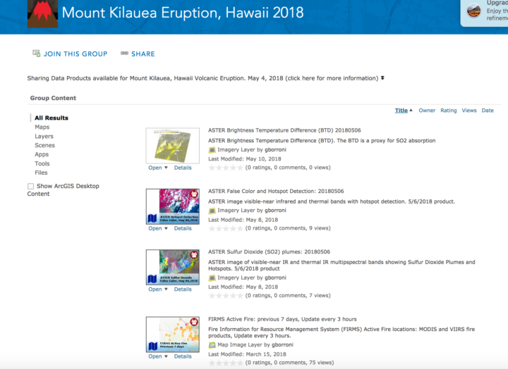
A screenshot from a repository of maps and images related to the eruption compiled by the NASA Earth Science Disasters Program. Image Credit: NASA
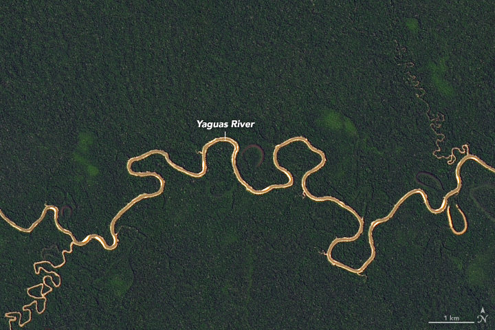
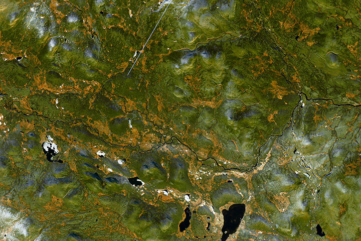
In January 2018, Peru’s protected area grew by more than 2 million acres with the creation of Yaguas National Park. The forest is largely intact, unbroken by roads and human activity. Only the Yaguas River cuts through the continuous canopy, visible in this image acquired by Landsat 8 in August 2017.
Scientists from the Field Museum got an even closer look at the forest when they flew over it before it was designated a national park. “When you see it from the air, it appears to stretch to the horizon,” said Corine Vriesendorp, a conservation ecologist at the Field, in a story about the new park. The following photographs by Álvaro del Campo offer this aerial perspective.
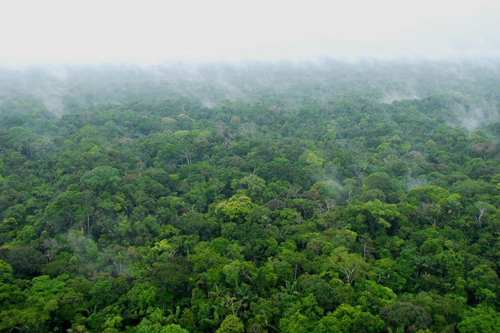
The first photo shows an area of intact forest inside Yaguas National Park. Expanses like this one are important for the diversity of the region’s plants and animals.
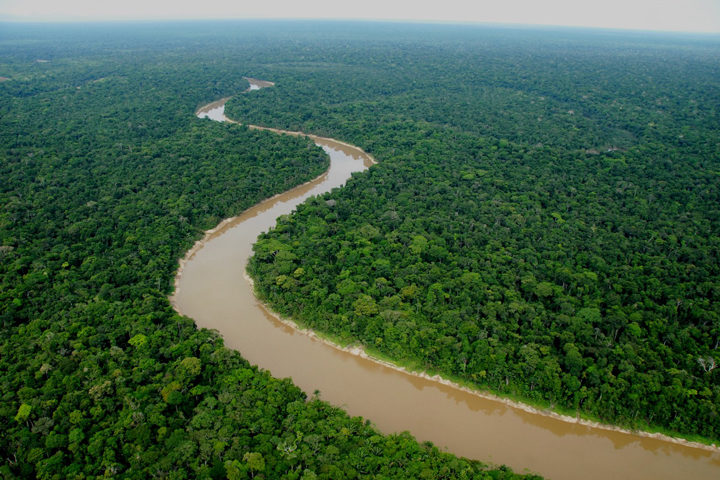
The park preserves more than forest; it protects an entire watershed. A segment of the Yaguas River is visible in the the second photograph. According to an inventory conducted by the Field Museum in 2010, the diversity of fish in this river could be the highest in Peru. Over the span of three weeks, experts counted 337 species of fish.
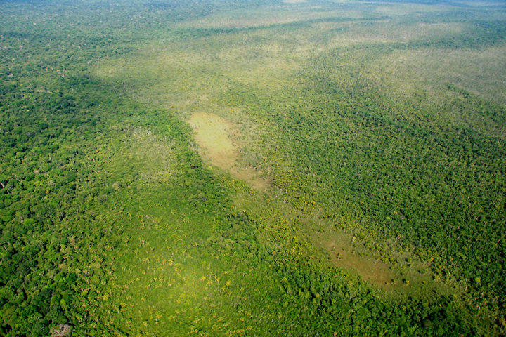
In the satellite image at the top of this page, notice the yellow areas on either side of the river that appear to be bare. These are actually peatlands: grounds rich with a soil-like mixture of partly decayed plant material that can build up in the abandoned river meanders. The photograph above provides an aerial view of peatlands.
“Ten years ago, we were just beginning to realize that there were important peat deposits in the Peruvian Amazon,” Vriesendorp said in a March 2018 Image of the Day. “Although there has been no comprehensive mapping of the Putumayo’s peatlands to date, it is likely that the below-ground carbon stock is immense.”
