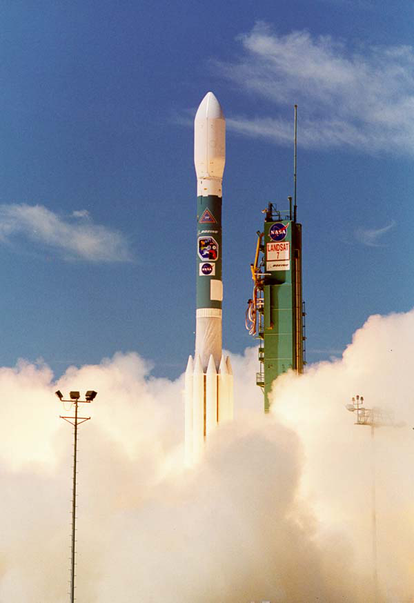
On April 15, 1999, Landsat 7 first made its way into space. 106,380 orbits later, the 2.6 million images acquired by Landsat 7 have given us a fuller and more nuanced understanding of Earth.
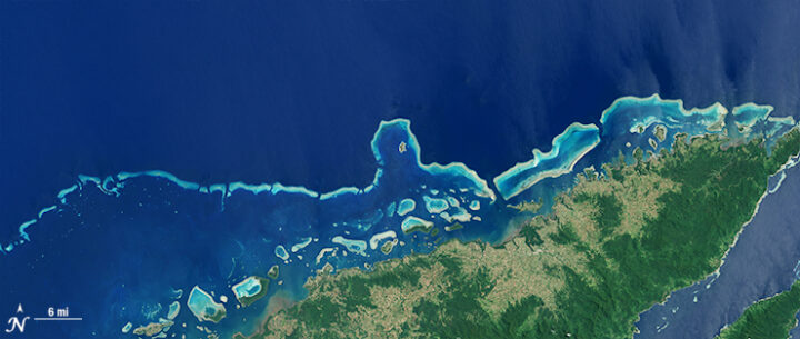
Take for example the Millennium Coral Reef Mapping Project. In 2006, Landsat 7 data were used to create a first-of-its kind global survey of coral reefs. The research lead on this project, Frank Muller-Karger, commented in 2015: “Until we made the map of coral reefs with Landsat 7, global maps of reefs had not improved a lot since the amazing maps that Darwin drafted.”
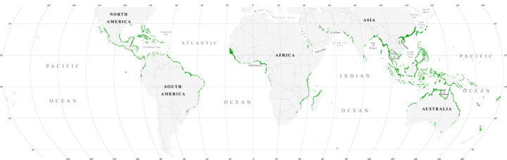
Landsat 7 data, together with data from its predecessor Landsat 5, provided the most comprehensive assessment ever of Earth’s mangroves in 2010.
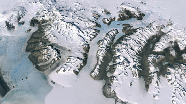
And for the International Polar Year (2007-2008), data from more than 1,000 Landsat 7 images were used to create the Landsat Image Mosaic of Antarctica (LIMA)—what was then the most detailed satellite mosaic of Antarctica.
If we travel two decades back in time and rewind the 4,733,375,587.686 kilometers that Landsat 7 has flown since April 1999, we arrive at a very different moment in spaced-based Earth observation.
The commercially-owned Landsat 6 satellite had failed to reach orbit six years earlier. Landsat 5 was 12 years past its design life and operated by a for-profit entity that charged upwards of $4000 per image and collected international data only when there was an immediate customer. Both situations curtailed the systematic global coverage of Earth that had been envisioned by the Landsat Program’s founders.
A building consensus about the critical role of Earth observation data for global change research had led the National Space Council to recommend that Landsat 7 be built. It should be operated by the U.S. government to ensure a continuous global archive of medium-resolution data for the long-term monitoring of Earth’s land surface. This was codified with the 1992 U.S. Land Remote Sensing Policy Act.
When Landsat 7 launched on April 15, 1999, the Enhanced Thematic Mapper Plus (ETM+) instrument onboard was the most sophisticated Landsat sensor yet. ETM+ carried a new 15-meter panchromatic band and had a thermal band with a spatial resolution refined to 60 meters (compared to 120 meters for Landsat 4 and 5). It also carried a new solid-state data recorder—one of the first to fly on a civilian mission. For the first time in Landsat program history, Landsat 7 was equipped with hardware that could reliably store large amounts of imaged data onboard for later download when a ground station was in range.
Landsat 7’s state-of-the-art recorder, together with a strategic global image acquisition plan, enabled the best global coverage the program had ever known. The LIMA project lead, Robert Bindschadler, penned in a 2001 journal article that “The revolutionary concept of systematic collection of Landsat 7 data timed to optimize anticipated scientific applications will make possible a global monitoring of the cryosphere with a data set heretofore only available in limited regions.”
During its ascent into orbit in 1999, Landsat 7 collected data as it flew under Landsat 5. This enabled the cross-calibration of Landsats 5 and 7. (In 2013, Landsat 8 underflew Landsat 7 for the same reason). Additionally, a team of calibration scientists oversaw in-the-field calibration efforts, making certain that satellite measurements agree with physical ground measurements. Such careful data calibration ensures that the Landsat data record can show meaningful trends of land use and land cover change—even when the changes are subtle.
In May 2003, an image scanning mechanism on Landsat 7 (the Scan Line Corrector) failed, leaving wedge-shaped gaps in the imagery—a net loss of 22 percent of each image. As devastating as this failure was, the remaining data are, as USGS describes, “some of the most geometrically and radiometrically accurate of all civilian satellite data in the world.”
The landmark 2008 USGS decision to make all Landsat data free and open, and the subsequent trend towards best-pixel composite-based data analysis, has made these data gaps even less problematic.
All in all, Landsat 7 has made remarkable contributions to global studies for two decades now, and according to fuel-based predictions, it should be able to continue doing so until the launch of Landsat 9.
In the second it took you to read this line, Landsat 7 traveled about 7.499 kilometers.
The launch of Landsat 7 was the second image ever posted on NASA Earth Observatory.
The Landsat 7 Mission Operations Control Center is staffed by 14 engineers, seven days a week, 8 hours a day. Someone is always on call and ready to respond if a ground or spacecraft anomaly occurs.
References:
Goward, S.N. et al. (2017) Landsat’s Enduring Legacy: Pioneering Global Land Observations from Space. Bethesda, MD: American Society for Photogrammetry and Remote Sensing.
Wulder, M.A. et al. (2019) “Current status of Landsat program, science, and applications.” Remote Sensing of Environment 225:127-147.

What do you get when you mix science with sugary marshmallow candy? Peepola Tesla, the candy bunny that invented the transmitter. Or Neanderpeeps, the group of sweet marshmallows that created fire. Or Dmitri Mendelpeep, the father of the peepiodic table.
For the first time possibly ever, science writers, school children, and enthusiastic science fans participated in “The World’s Finest Science-Themed Peeps Diorama Contest.” Participants were asked to recreate scenes of scientific discoveries, field work, moments in history, and model organisms— all made with the spring marshmallow treats. With nearly 50 entries to choose from, you now get to vote on which diorama deserves the coveted “Peeple’s Choice Award.”
Of course here at NASA Earth Observatory, we are partial to the space- and Earth-themed dioramas. Take a peep at some of the entries below. Make sure to vote for your favorite here before April 14, 2019.

Antarctic peep-searchers use Landsat images of peep-guin peep (er, poop) to measure the health of colonies. Penguin peep (er, poop) is bright pink and bright blue, depending on if they’re eating shrimp or sardines. What they’re eating and how much peep (er, poop) is on the ice is an important indicator of peep-guin health. In this diorama, intrepid peep-searchers are bundled up in their cozy Arctic gear, visiting the peep-guin colony from a peep-search ship to ground-truth the colony counts they’re getting with satellite data. Reminder to all peep-searchers: Don’t eat the pink snow!
Read about the original research on NASA Earth Observatory.

Peep scientists are investigating an unusual object at the far reaches of the solar system, known as Ultima Peep. The spacecraft New Hare-rizons is closing in, and images of Ultima Peep are becoming clearer. At first, Ultima Peep appeared to be shaped like a bowling pin, but now, some are beginning to suspect that Ultima Peep is shaped like a peep. (Perhaps it is a lonely space peep?) The peeple demand information! Scientists have called a press conference to weigh in, and journalists are peepering them with questions.
The scientific inspiration for this diorama is, of course, NASA’s New Horizons spacecraft and its investigation of the Kuiper Belt object Ultima Thule, the shape of which became clearer as the spacecraft got closer. Unfortunately, in our world, bunny ears never materialized. The diorama also includes a title and a close-up of the encounter between New Hare-rizons and Ultima Peep.
Read about the Ultimate Thule flyby.
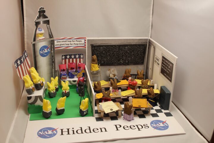
Hidden Peeps is an artistic rendering of the Black women who made essential contributions to the U.S. scientific space program at NASA. The right side of the diorama depicts the women, known as computers, whose work enabled US spaceflights but went largely unsung. The details include Dorothy Vaughan programming an early computer, Katherine Johnson and Mary Jackson writing their official technical reports, other women doing math on the chalkboard, calculating trajectories, verifying fight patterns. Be sure to check out the ‘colored’ bathroom sign (NASA’s facilities in Virginia were segregated), the Mary Jackson quote, the women’s glasses, typewriter, pencils, coffee mugs and family peeps photo.
The other side of the diorama depicts the men receiving attention and accolades for the space program complete with astronaut John Glenn in the rocket, military band, NBC photographer, and medals. Check out the NASA logo and the Neil Armstrong-inspired banner, “One small hop for Peeps….”
Learn more about NASA’s Hidden Figures and Modern Figures.
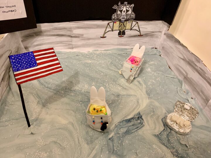
Astropeeps Bunny Aldrin and Neil Peepstrong explore Tranquilipeep Base — making history as the first sentient marshmallows to step on the moon. Marshmallow Collins drew the short straw and is orbiting up high in the Columbia capsule.
Meanwhile, Bunny is collecting rock samples with his shovel and sample box, and Neil takes pictures with his hand-held camera. The two astropeeps have already planted the American flag, and their ride — the Eagle lander — waits in the distance. They keep their spacesuits on, because bad things happen to Peeps in a vacuum…
See the photograph taken by Neil Armstrong of the Lunar Module at Tranquility Base.
Peepil Armstrong takes his first hop on the moon.
View the original video of Neil Armstrong walking on the moon.

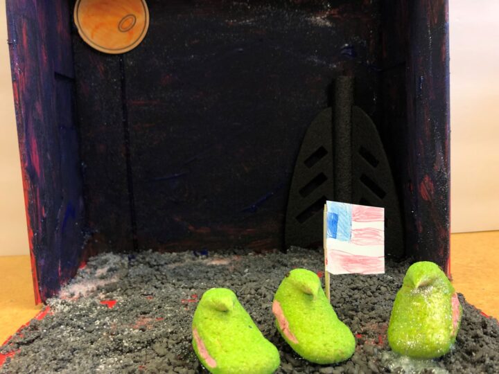
Wernher Von Braun’s V2 rockets ultimately powered the Saturn V and took the United States to the moon, but von Braun always saw Mars as the true destination. Today, we are proving him right. So while the crowds have their eyes on the moon, von Braun points the way to Mars.
Learn about NASA’s mission to Mars.
The contest is hosted by The Open Notebook, a non-profit publication aimed to help science journalists sharpen their skills by providing useful tools, articles, and career advice. The contest is the brainchild of volunteers Joanna Church, Helen Fields, and Kate Ramsayer, an award-winning trio of peep diorama makers from the Washington, DC, area.
On February 12, 1809, Charles Robert Darwin was born in England in the town of Shrewsbury. The famed naturalist, geologist, and biologist is best known for his 19th century expedition to the Galápagos Islands, which inspired revolutionary insights about evolution and natural selection. Lesser known is that the expedition to the Galápagos was just one part of a much longer journey. The Second Voyage of the HMS Beagle brought Darwin and his fellow travelers to South America, Australia, Africa, and several islands in between. Here are a few interesting places where the HMS Beagle stopped that we have covered in earlier stories.
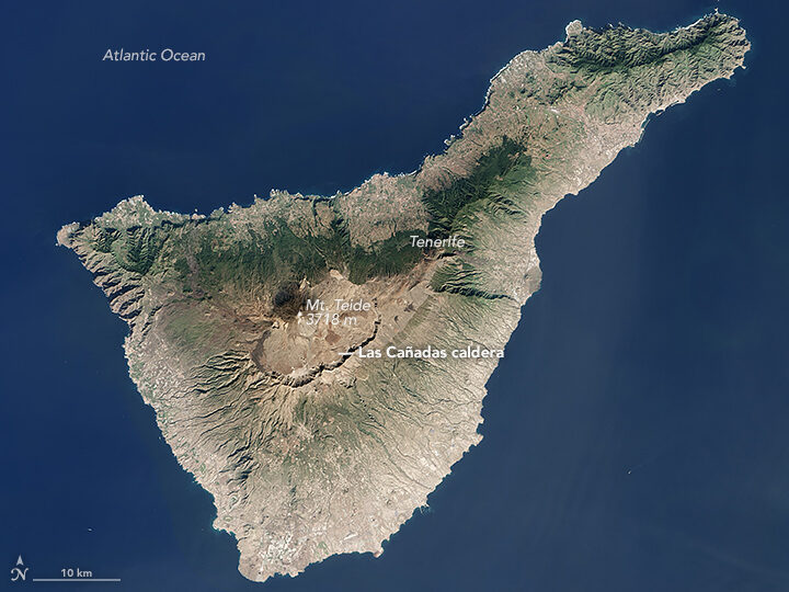
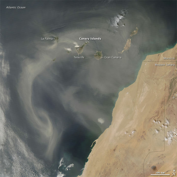
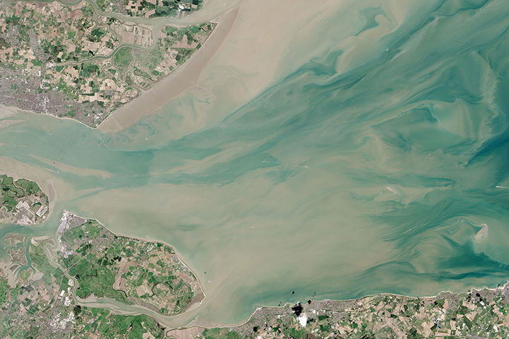
The crew of the Beagle was denied landing on Tenerife because of fears they might be carrying cholera. The Operational Land Imager (OLI) on Landsat 8 acquired this image of the island on January 25, 2016.
Darwin was struck by the intensity of the dust in this area. “The atmosphere is generally very hazy, chiefly due to an impalpable dust, which is constantly falling, even on vessels far out at sea,” he wrote. “It is produced, as I believe, from the wear and tear of volcanic rocks, and must come from the coast of Africa.”
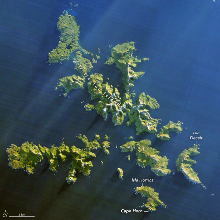
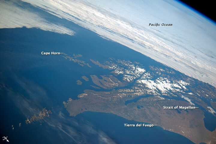
Southwest of Cape Horn at the southern tip of South America, the ocean floor rises sharply. Along with the potent westerly winds that swirl around the Furious Fifties, this pushes up massive waves with frightening regularity. Add in frigid water temperatures, rocky coastal shoals, and stray icebergs—which drift north from Antarctica across the Drake Passage—and it is easy to see why the area is known as a graveyard for ships. In his journal, Darwin described the harrowing journey as the explorers tried to round the Horn just before Christmas.
“Great black clouds were rolling across the heavens, and squalls of rain, with hail, swept by us with such extreme violence, that the Captain determined to run into Wigwam Cove. This is a snug little harbor, not far from Cape Horn; and here, at Christmas-eve, we anchored in smooth water. The only thing which reminded us of the gale outside, was every now and then a puff from the mountains, which made the ship surge at her anchors.”
Charles Darwin
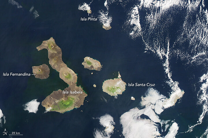
The Galapagos archipelago includes more than 125 islands, islets, and rocks populated by a diversity of wildlife. Charles Darwin’s book, The Voyage of the Beagle, cast a spotlight on the Galapagos, which he called “a little world within itself, or rather a satellite attached to America, whence it has derived a few stray colonists.” It was this little world that would revolutionize scientific understanding of biology and lead to Darwin’s On the Origin of Species, which would come to be known as the foundation of evolution.
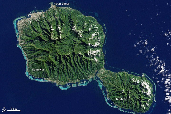
On this stopover, Darwin had a chance to explore coral reef.
“We paddled for some time about the reef admiring the pretty branching Corals,” he wrote. “It is my opinion, that besides the avowed ignorance concerning the tiny architects of each individual species, little is yet known, in spite of the much which has been written, of the structure and origin of the Coral Islands and reefs.”
The Enhanced Thematic Mapper Plus on the Landsat 7 satellite captured this natural-color image of Tahiti on July 11, 2001. This island is part of a volcanic chain formed by the northwestward movement of the Pacific Plate over a fixed hotspot.
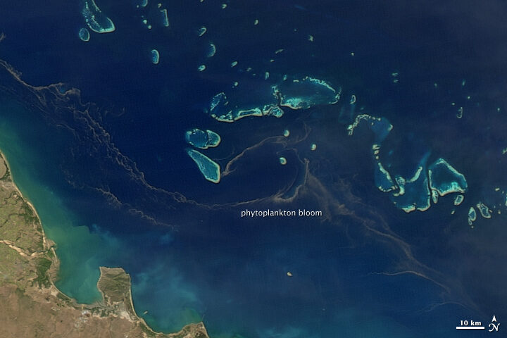
All the sea travel offered plenty of time to observe and ponder the intricacies of phytoplankton.
“My attention was called to a reddish-brown appearance in the sea. The whole surface of the water, as it appeared under a weak lens, seemed as if covered by chopped bits of hay, with their ends jagged,” he wrote. “These are minute cylindrical, in bundles or rafts of from twenty to sixty in each…Their numbers must be infinite: the ship passed through several bands of them, one of which was about ten yards wide, and, judging from the mud-like color of the water, at least two and a half miles.”
On August 9, 2011, the Moderate Resolution Imaging Spectroradiometer (MODIS) on the Aqua satellite captured this image of a similar band of brown between the Great Barrier Reef and the Queensland shore. Though it’s impossible to identify the species from satellite imagery, such red-brown streamers are usually trichodesmium. Sailors have long called these brown streamers “sea sawdust.”
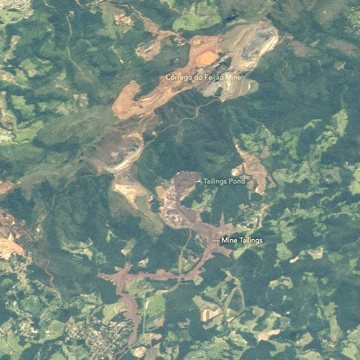
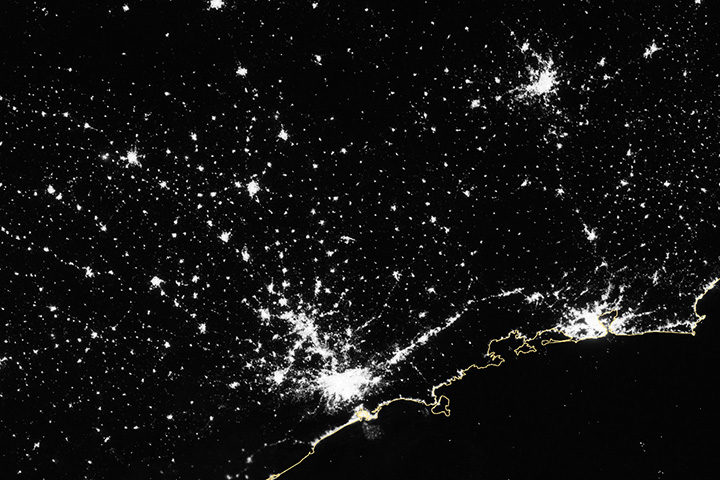
A few days after we published a Landsat 8 image of a deadly dam collapse and flood in Brazil, astronauts photographed the scene from the International Space Station on February 2, 2019.
The tailings pond label points to the source of the mine waste. When an earthen dam on the southwestern edge of that pond collapsed on January 25, it sent a torrent of sludge pouring down a valley toward the Paraopeba River. Over a distance of roughly 8 kilometers (5 miles), the mine sludge overran the mine’s headquarters, a hotel, and a residential area. Videos published by news agencies and AGU’s Landslide Blog offer a remarkable view of the dam collapsing and sludge rushing forward at roughly 120 kilometers (75 miles) per hour.
NASA’s Earth Science Disasters Program has developed an interactive version of the astronaut photograph that allows you to explore the area before and after the disaster. More astronaut photos of the event are available here.

The Telstar satellite (left) and the 1974 Telstar Durlast, the official ball of the 1974 World Cup. Image Credit: Bell Labs/Shine 2010
Goooooooal!!!! The 2018 FIFA World Cup kicked off on June 14, 2018.
Here’s a bit of Cup trivia you may not know. In 1962, NASA launched a small, spherical communications satellite called Telstar that ended up altering the look of the balls used in the World Cup.
Telstar was the first active communications satellite and the first commercial payload in space. By sending television signals, telephone calls, and fax images from space, the 3-foot-long satellite kicked off a whole new era in telecommunications—and soccer ball design.
There’s a direct line between the distinctive black and white patterning of Telstar’s hull and solar panels and the Adidas ball used as the official ball of the 1970 World Cup in Mexico and the 1974 World Cup in West Germany. While earlier generations of soccer balls were brown and did not show up well on television, the 1970 and 1974 balls featured the now iconic 32-panel design of alternating white hexagons and black pentagons, a pattern that closely resembled Telstar. Fittingly, that first ball was called Telstar Elast; the official ball in 2018, a nod to the 1970 ball, is called the Telstar 18.
To celebrate the World Cup, Earth Observatory is planning to dig into its archives. For key games, we’ll grab one image for each of the two countries going head to head. Can you guess which image goes with which country? Just click on the images below to find out. Enjoy the tournament!
June 14:
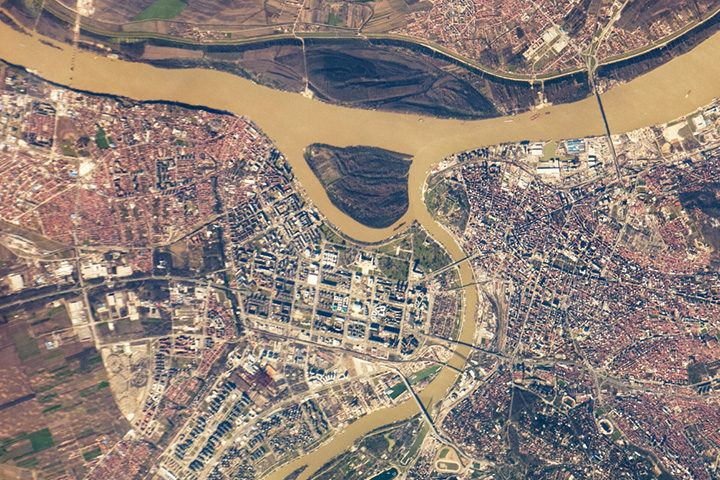
Russia 5 — 0 Saudi Arabia

June 15
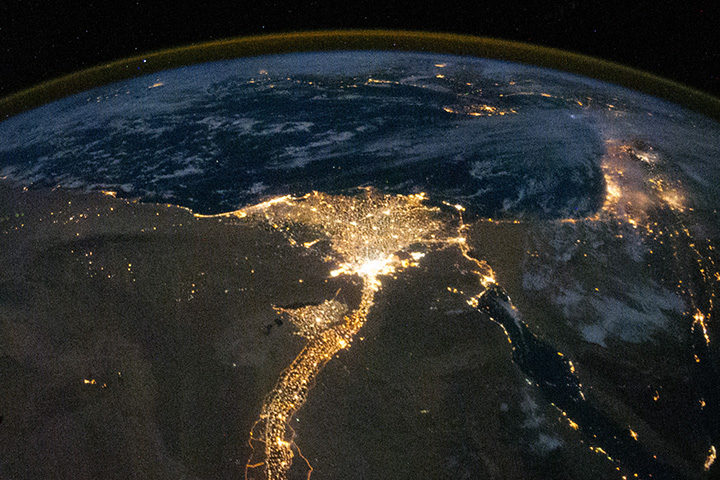
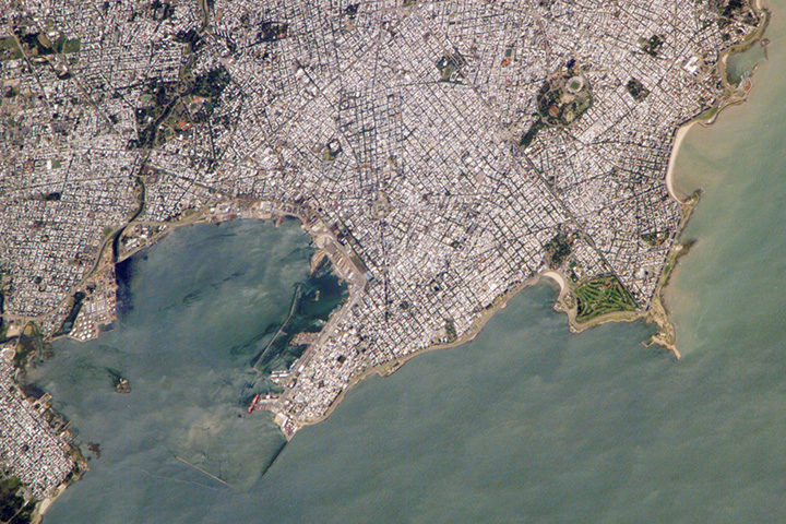
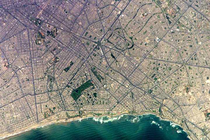
Uruguay 1 — 0 Egypt
Iran 1 — 0 Morocco
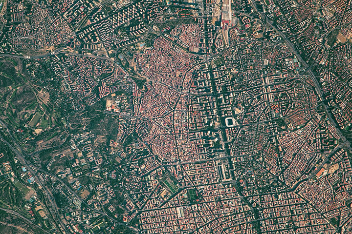
Portugal 3 — 3 Spain
June 16
France 2 — 1 Australia
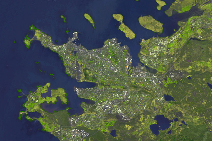
Iceland 1 — 1 Argentina
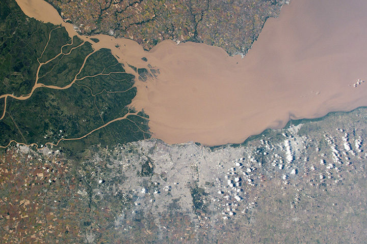
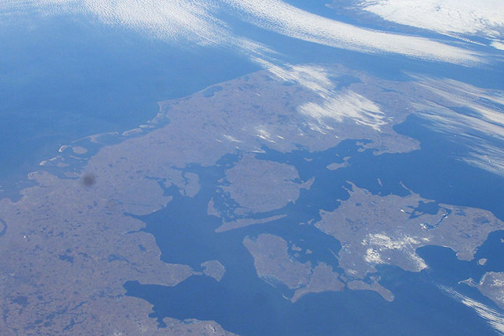
Peru 0 — 1 Denmark
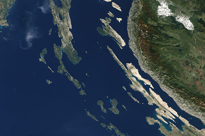
Croatia 2 — 0 Nigeria
June 17
Costa Rica 0 — 1 Serbia
Brazil 1 — 1 Switzerland
Mexico 1 — 0 Germany
June 18
Sweden vs. Korea Republic
Belgium vs. Panama
Tunisia vs. England

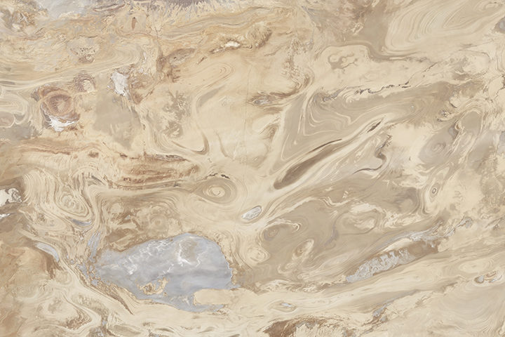
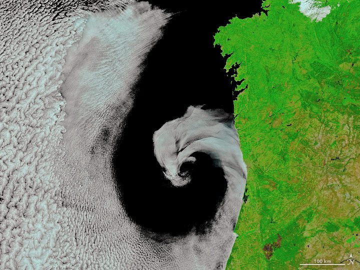
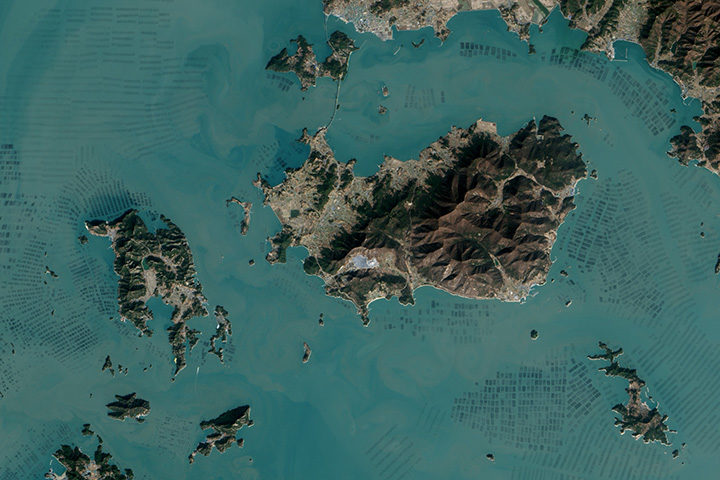
Every month on Earth Matters, we offer a puzzling satellite image. The November 2017 puzzler is above. Your challenge is to use the comments section to tell us what we are looking at, when the image was acquired, and why the scene is interesting.
How to answer. You can use a few words or several paragraphs. You might simply tell us the location. Or you can dig deeper and explain what satellite and instrument produced the image, what spectral bands were used to create it, or what is compelling about some obscure feature in the image. If you think something is interesting or noteworthy, tell us about it.
The prize. We can’t offer prize money or a trip to Mars, but we can promise you credit and glory. Well, maybe just credit. Roughly one week after a puzzler image appears on this blog, we will post an annotated and captioned version as our Image of the Day. After we post the answer, we will acknowledge the first person to correctly identify the image at the bottom of this blog post. We also may recognize readers who offer the most interesting tidbits of information about the geological, meteorological, or human processes that have shaped the landscape. Please include your preferred name or alias with your comment. If you work for or attend an institution that you would like to recognize, please mention that as well.
Recent winners. If you’ve won the puzzler in the past few months or if you work in geospatial imaging, please hold your answer for at least a day to give less experienced readers a chance to play.
Releasing Comments. Savvy readers have solved some puzzlers after a few minutes. To give more people a chance to play, we may wait between 24 to 48 hours before posting comments.
Good luck!
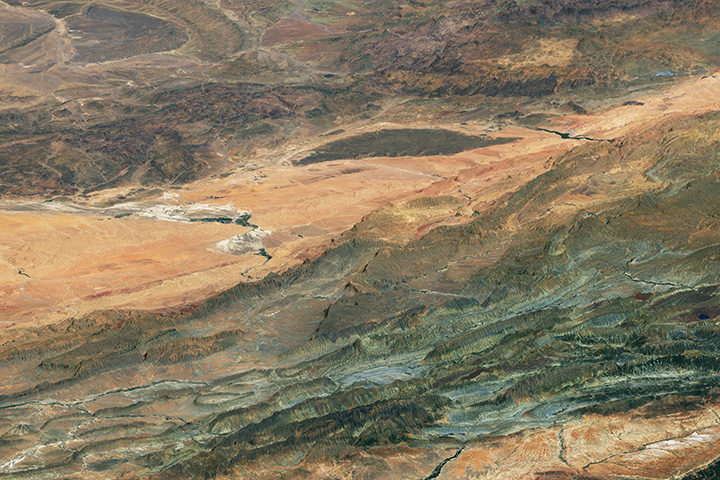
In this satellite image, the prominent Pinacate Peaks stick out above the sand dune landscape of the Gran Desierto de Altar in Mexico’s Sonoran Province. The peaks are located just south of the Mexico-United States border. The Gran Desierto de Altar is one section of the broader Soronan Desert which covers much of northwestern Mexico and reaches into Arizona and California.
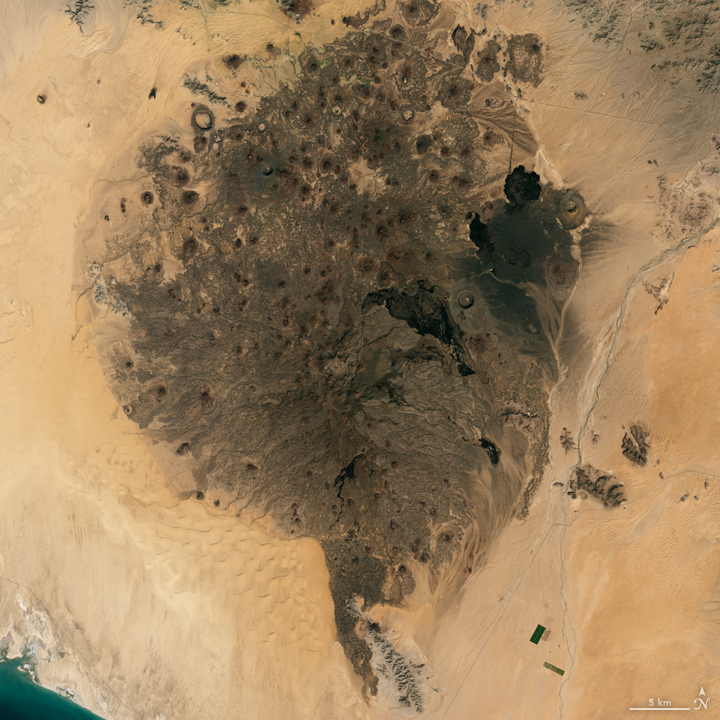
Steady, consistent winds in the area have shifted low-lying sand into dune fields in intriguing regular patterns. These same patterns of sand dune fields appear around the world in desert areas.
The volcanic peaks and cinder cones are believed to have formed from volcanic activity that first started roughly 4 million years ago — most likely due to the plate tectonics that also formed the Gulf of California around the same time. The most recent activity was perhaps 11,000 years ago. During the late 1960s, NASA trained astronauts in field geology at a number of sites around the world, including Pinacate Peaks, as preparation for the lunar landings.
The natural color image here is from the Landsat 8 satellite using its Operational Line Imager (OLI) instrument. The image was acquired on October 3, 2017. The volcanic cinder cone field stains the landscape of bright sand and tall dunes in the El Pinacate y Gran Desierto de Altar Biosphere Reserve.
NOTE: In a previous version of this post, I featured the EO-1 ALI image below, and an astute reader pointed out that these peaks, while in the Biosphere Reserve, are not Pinacate Peaks, but rather the Sierra de Rosario range nearby. I am geographically and tectonically embarassed…
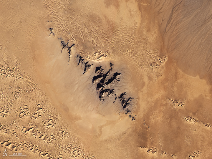
The natural color image here is from the now-defunct Earth Observing 1 (EO-1) satellite using its Advanced Land Imager (ALI). The image was acquired on December 16, 2012. This late-year scene was just days before the solstice (the farthest south the Sun appears in the sky), so the tallest sand dunes and the volcanic peaks cast unusually long shadows across the ground.
EO-1 was launched in November 2000 as an engineering testbed for new sensor technology; in particular, the ALI instrument was a predecessor for the Landsat 8 Operational Land Imager. The EO-1 mission was so successful that it was extended past its original 18-month mission, and was only recently retired after 17 years of operation.
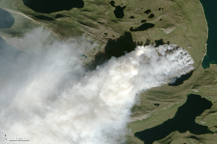
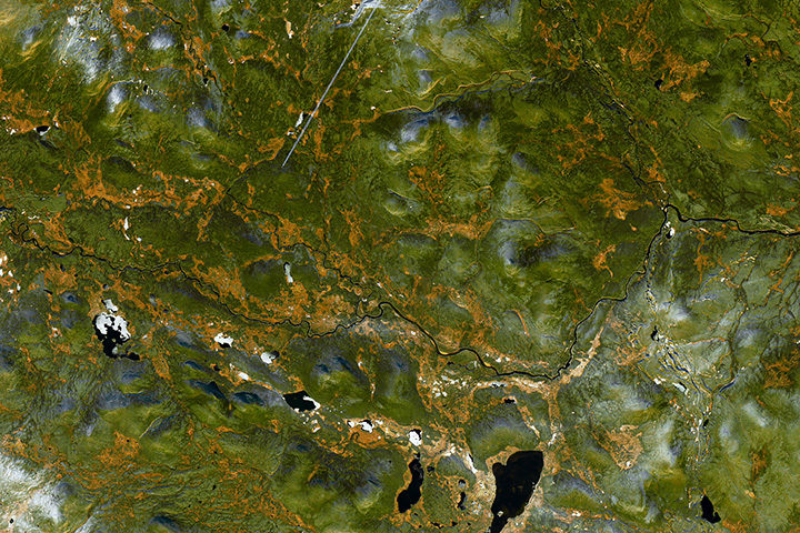
NASA Earth Observatory image by Jesse Allen, using Landsat data from the U.S. Geological Survey. The image was captured on August 3, 2017, by the Operational Land Imager (OLI) on Landsat 8.
Scientists around the world have been using satellites to monitor a wildfire in Greenland. In a place better known for ice, just how unusual is this fire? NASA Earth Observatory checked with Earth science experts Ruth Mottram, Jessica McCarty, and Stef Lhermitte to find out. Mottram is a climate scientist at the Danish Meteorological Institute; Lhermitte is remote sensing scientist at Delft University of Technology; and McCarty is a geographer at Miami University.
How unusual is this fire?
Mottram: Many of my colleagues at the Danish Meteorological Institute (DMI) were a bit surprised at first, but it was clear talking to both the Greenland weather forecasters (they do three month rotations to the airport at Kangerlussuaq) and to some of the older guys that fires do happen reasonably regularly, particularly in the west and south. However, they are not always reported either officially or in the news unless the fire is close to a settlement or affecting shipping or flights. This fire seems to be a fairly large one, but there has been no systematic attempt to gather evidence or data on Greenland’s fires – at least not at DMI. I have never heard of anyone else in Denmark doing it either, so it is a bit hard to be more precise than that.
McCarty: This is a hard question to answer, and I keep telling media reporters the same thing: we need to have the wildfire history analyzed before we know how unusual this is. I can tell you from the global wildfire science community that I am a part of, we would have never thought the we would need to make a wildfire history to understand the fire regime in Greenland. So that part is unusual.
Lhermitte: I completely agree with Jessica. I used to be a wildfire remote sensing scientist (finished my PhD on African wildfires in 2008), but I have shifted since then to the cryosphere community (including some work on Greenland’s ice). It was a big surprise to me to see both worlds combined on Monday when I first noticed a Greenland fire tweet. Now it is clear that fires have occurred before, but that we basically lack a good record. MODIS gives us a glimpse, but the sensor cannot detect fires through clouds, and the record is short. Based on what I have seen, the 2017 fire is the biggest one on the MODIS record, but the record is sparse and incomplete.
I know you have done some looking through MODIS and Landsat satellite data for evidence of past fires in Greenland. What have you found?
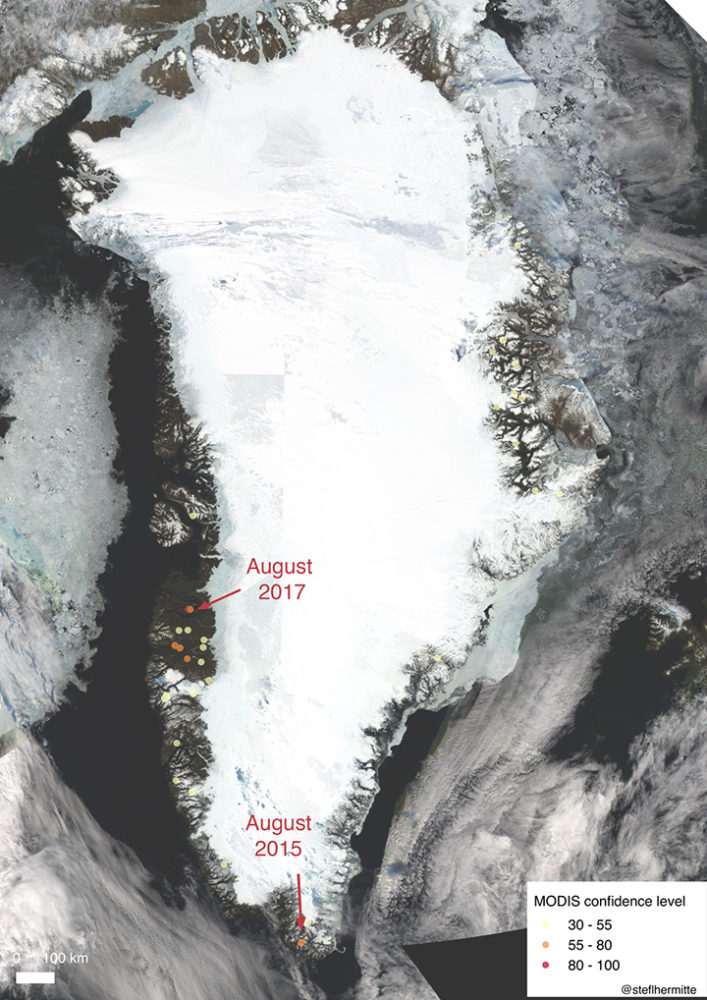
Lhermitte: I looked back at the record of MODIS active fire detections since 2002 and made a quick overview map. In the map below, fire detections are marked with circles. Higher confidence fires are red; lower confidence fires are yellow. In most years, the satellite flags about 5 pixels as having active fires. In 2015, it flagged about 20 pixels. There were over 40 pixels flagged in 2017, so this year has been exceptional. Note: Most of these detections are probably campfires or false detections—not uncontrolled wildfires. There have been two big wildfires: the one happening now and one in August of 2015.
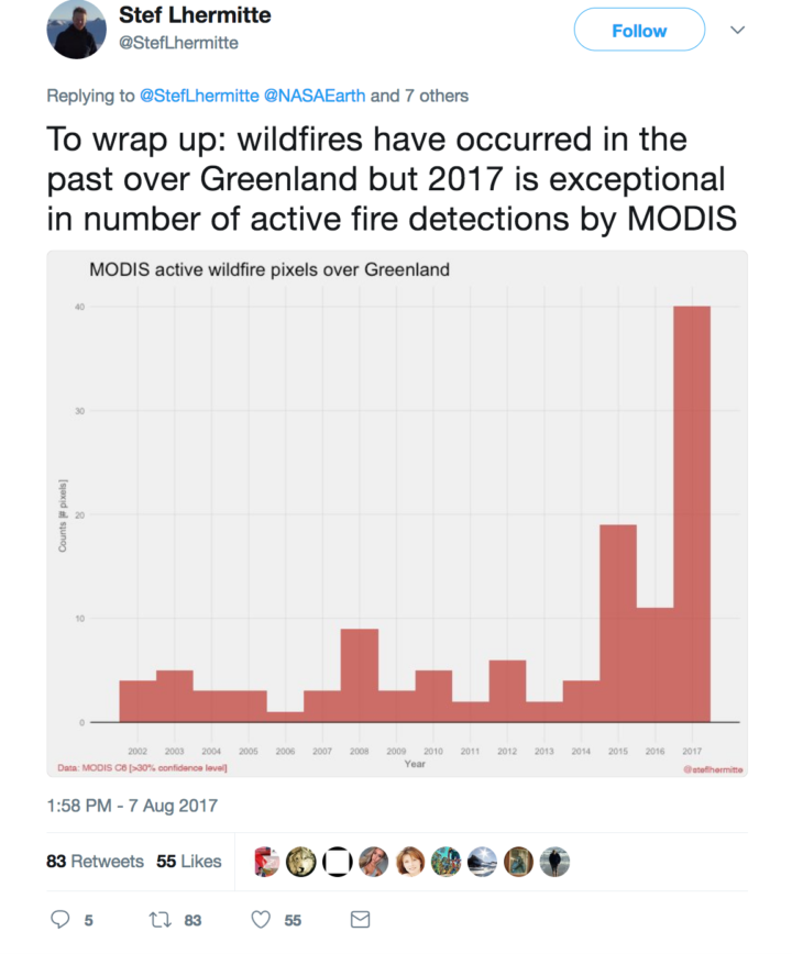
McCarty: Overall, 2017 appears to be a larger fire season than any year since 2001. But from a remote sensing point of view, this is a difficult place to study the fire regime using satellite-based active fire detections (because of cloudiness and other factors). The Landsat/Sentinel-2/Deimos, etc. burn scar images will be more helpful.
Mottram: I have not looked into any of the specific data, but I have heard anecdotes about fires in Narsarsuaq close to the DMI ice service reconnaissance station in the south of Greenland, in the Kobbefjord close to Nuuk, and just to the north of Sisimiut near this one. There was also a large fire in 2008 near Eqi, close to Ilulissat, which the Greenland press reported was caused by a tourist burning rubbish but failing to put the fire out.
One of you said on social media that you think the fire may be burning through peat. Are you sure? How can you tell?
McCarty: The fire line has not moved much in comparison to a wildfire in a grassland or forest. However, Stef made an awesome Sentinel-2 animation that shows the fire line moving some. I still think it is peat with a mix of grasses and moss (given the Google Earth Pro and Deimos imagery), but how deep the peat is difficult to ascertain. A recent study in the Qaanaaq region (north of where these wildfires are) found five times more peat in the soil distribution and soil content than previously reported. Also, historically, peat houses were constructed in this area of Greenland, which means there are peat deposits nearby. Short grasses with underlying peat is my working hypothesis for now since we are onto day 11 of the fire.
Mottram: I am not really a soils expert, and Greenland really suffers from having little detailed mapping of this kind. Also, Greenland is pretty diverse from north to south and east to west. There are high rocky mountains and permafrost. The south has sheep pasture and even some areas of forest; the north has large areas with low vegetation cover. However, there are also extensive areas of peat cite in the scientific literature.
Do you think this fire was triggered by human activity or lightning? Do we know what triggers most fires in Greenland?
McCarty: I still can’t find any indication that this was lightning, so it must be human activity. Greenlandic/Danish news reports are reporting that hikers and tourists should stay from this area, so I would assume that humans are on the landscape there.
Mottram: I can’t really say for sure. Lightning is not impossible, but neither is human activity. It is the middle of the hunting/fishing/berry-picking/hiking season, and this area is known for reindeer. In fact, the Greenland press had an interview with a reindeer hunter who had to turn back from visiting because of the smoke in the fjord. Actually, the hunter wanted the fire put out by the authorities, so he could go hunting there.
What has the weather been like in Greenland during the last few months? Has it been unusually hot or dry where this fire is burning?
Mottram: It has been a very dry summer in the south but also quite dry in this region, and the fire was preceded by some relatively high temperatures. My climatologist colleague John Cappelen tells me that the DMI station at Sisimiut measured an precipitation anomaly of -30.0 millimeters for June and -20.7 millimeters for July compared to the mean precipitation of 1981-2010. In other words, there was almost no rain in June and a bit more than half the usual rainfall in July. There have also been some warm days in Sisimiut (or at least at the airport where the weather station is), particularly towards the end of the month. The monthly average temperature was 7.1 Celsius compared to a 1961-1990 average of 6.3 Celsius in July. The trend has continued into August as well.
This fire got me wondering why there are ice-free areas along Greenland’s coast where vegetation grows. Are these relatively new features? How do you think they got there?
Lhermitte: These ice free coastal areas are mainly the result of the bedrock topography, where the coastal Greenland areas are much more elevated than the interior of Greenland. Since the last glacial maximum, the ice sheet has partly retreated and exposed more land. If the ice sheet would retreat further, we would see more of the inner, lower land exposed.
Mottram: The ice sheet is more or less in equilibrium with the climate, so it is where it is because that is where the glaciers can flow. During the last glacial maximum, the ice sheet extended far out onto the continental shelf and connected (in the north west) with the Laurentide ice sheet in North America. Then, with warming after the last glacial period, the ice sheet retreated. (That is, more ice was melting and calving away than was being replenished by snowfall.) The ice sheet has been more or less stable in its present extent for about the last 10,000 years (with some smaller advances and retreats responding to more local climate variability).
Summer is beach season in the northern hemisphere. But even if you’re a regular at your local swimming hole, you probably haven’t seen too many beaches from this perspective. This video from NASA Earth Observatory shows the satellite and space-station view of various shorelines across the United States. No sunblock necessary.
It takes a certain amount of devotion to reach Miyar Glacier. The glacier sits high in the Indian Himalayas, well away from towns and roads, but it rewards explorers with stunning scenery and mountain peaks that rise above 6,000 meters (20,000 feet). Many of the peaks have little or no record of previous ascents. Satellites, however, can explore with considerably greater ease.
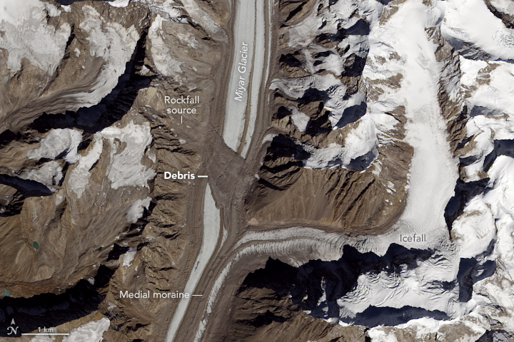
The Operational Land Imager (OLI) on Landsat 8 acquired this image on October 19, 2016. Summer warmth had melted off snow from the previous winter, leaving only the permanent snow and ice cover. Notice the debris field spread across the width of the glacier. The landslide that left it predates this image by some time; we know this because the debris has been carried downstream by the flow of the ice.
A little exploring with the Google Earth Engine timelapse tool shows Landsat 8’s high dynamic range — that is, its ability to discern both dim and bright features. In images prior to 2013, much of the glacier is featureless and white because it was too bright for the older Thematic Mapper (Landsat 5) and Enhanced Thematic Mapper Plus (Landsat 7) instruments to make out details. Images from 2013 onwards, which use the newer OLI data, show more detail. Still, it is fairly clear that there was no landslide feature as recently as 2007, and the slide definitely had taken place by 2010. Indian researchers used other satellite resources to pin the landslide date down to some time in 2009.
The Miyar Glacier has a relatively smooth surface in this image, with long linear streaks through the center of the glacier. These are medial moraines, features that form when two or more glaciers merge. The confluence of the tributary and the glacier shows how new material gets carried in to create medial moraines.
The tributary merging from the east (in the image above) shows choppy features from the confluence all the way upstream. This very rough surface is an icefall, a feature somewhat akin to rapids or a waterfall in a river. The glacier at the bend is roughly 700 meters (2,100 feet) higher than at the Miyar confluence (approximately 5,200 meters and 4,500 meters above sea level respectively). The ice is flowing over a rough and steep rock surface, causing matching rippling in the ice surface.
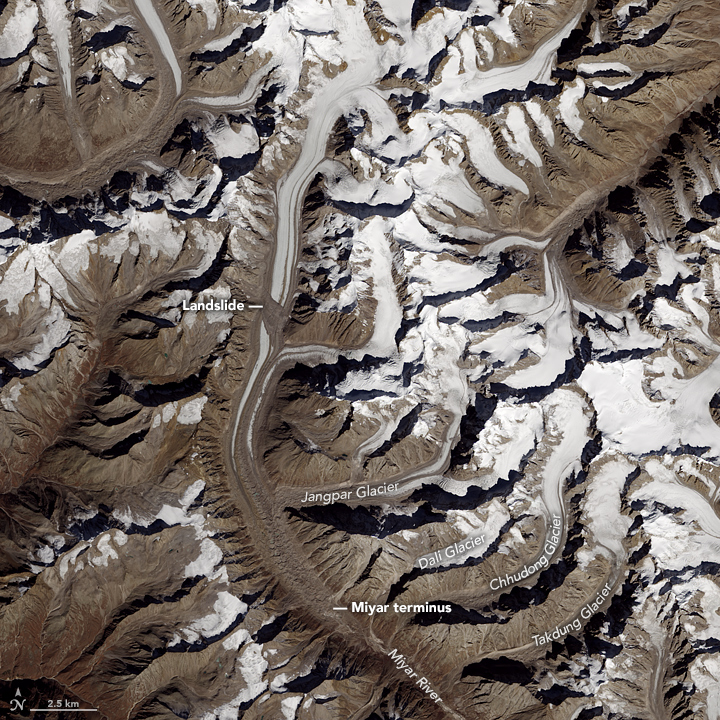
The wider image shows the terminus of the Miyar Glacier as well as a number of other tributary glaciers. The names shown here are based on the American Alpine Journal (2009), which notes that many of these glaciers have different names in trekking journals and maps.
