In July 2016, the lower portion of a valley glacier in the Aru Range of Tibet detached and barreled into a nearby valley, killing nine people and hundreds of animals. The huge avalanche, one of the largest scientists had ever seen, sent a tongue of debris spreading across 9 square kilometers (3 square miles). With debris reaching speeds of 140 kilometers (90 miles) per hour, the avalanche was remarkably fast for its size.
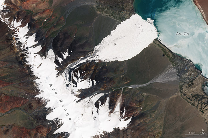
(NASA Earth Observatory image by Joshua Stevens, using modified Copernicus Sentinel 2 data processed by the European Space Agency. Image collected on July 21, 2016.)
Researchers were initially baffled about how it had happened. The glacier was on a nearly flat slope that was too shallow to cause avalanches, especially fast-moving ones. What’s more, the collapse happened at an elevation where permafrost was widespread; it should have securely anchored the glacier to the surface.
Two months later, it happened again — this time to a glacier just a few kilometers away. One gigantic avalanche was unusual; two in a row was unprecedented. The second collapse raised even more questions. Had an earthquake played a role in triggering them? Did climate change play a role? Should we expect more of these mega-avalanches?
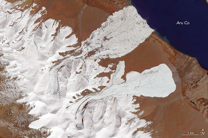
(NASA Earth Observatory image by Joshua Stevens and Jesse Allen, using ASTER data from NASA/GSFC/METI/ERSDAC/JAROS, and U.S./Japan ASTER Science Team. Image collected on October 4, 2016.)
Now scientists have answers about how these unusual avalanches happened. There were four factors that came together and triggered the collapses, an international team of researchers reported in Nature Geoscience. The scientists analyzed many types of satellite, meteorological, and seismic data to reach their conclusions. They also sent teams of researchers to investigate the avalanches in the field.
First, increasing snowfall since the mid-1990s caused snow to pile up and start working its way toward the front edge of the glaciers (a process known as surging). Second, a great deal of rain fell in the summer of 2016. As a result, water worked its way through crevasses on the surface and lubricated the undersides of the glaciers. Third, water pooled up underneath the glaciers, even as the edges remained frozen to the ground. Fourth, the glaciers sat on a fine-grained layer of siltstone and clay that became extremely slippery.
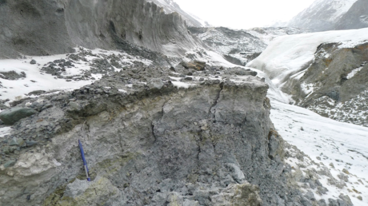
Notice the large amounts of silt and clay in the path of the first avalanche. (Photo taken on July 15, 2017, by Adrien Gilbert/University of Oslo)
Earth Observatory checked in with Andreas Kääb (University of Oslo), lead author of the study, to find out more about how the avalanche happened and what it means.
These glaciers were not on a steep slope, but the avalanche moved quite quickly. How did that happen?
Strong resistance by the frozen margins and tongues of the glaciers allowed the pressure to build instead of enabling them to adjust. The glaciers were loading up more and more pressure until the frozen margins suddenly failed. Local people reported a load bang. Once the margins failed, there was nothing at the glacier bed to hold it back, just water-soaked clay.
Your study notes that there was “undestroyed grassy vegetation on the lee side of the hills, suggesting that the fast-moving mass had partially jumped over it.” Are you saying the avalanche was airborne? If so, is that unusual?
Yes, for a small part of the avalanche path. We see this for other large-volume, high-speed avalanches, and it really illustrates the massive amount of energy released. You need quite high speeds in order for debris to jump. For us, the phenomenon is important as validation for the speeds obtained from the seismic signals the avalanches triggered and the avalanche modeling that we did.
Would you say these collapses were a product of climate change?
Climate change was necessary, but other factors that had nothing to do with climate were also critical. The increasing mass of the glaciers since the 1990s and the heavy rains and meltwater in 2016 are connected to climate change. The type of bedrock and the way the edges were frozen to the ground had nothing to do with climate change.
Can we expect to see more big glacial collapses as the world gets warmer?
It’s not clear. Climate change could increase or, maybe even more likely, decrease the probability of such massive collapses. Most glaciers on Earth are actually losing mass (not gaining, like the two glaciers in Tibet were). Also, if permafrost becomes less widespread over time and glacier margins melt, it is less likely that pressure will build up in that way that it did in this case.
I know you used several types of satellite data as part of this analysis. Can you mention a few that yielded particularly useful information?
We used a lot of different sources of data: Sentinel 1 and 2, TerraSAR-X/TanDEM-X, Planet Labs, and DigitalGlobe WorldView. Landsat 8 was absolutely critical because it gave the first and critical indication of the soft-bed characteristics. The entire Landsat series was instrumental for checking the glacier history since the 1980s. We also used declassified Corona data back to the 1960s.
Are these sorts of avalanches likely to happen in other parts of the world?
Honestly, I have no clue at the moment, but we would be much less surprised next time. We know now that this type of collapse can happen under special circumstances. (It happened once before in the Caucasus at Kolka Glacier.) One thing that should be investigated is whether there are other glaciers—especially polythermal ones—with these very fine-grained materials underneath them.
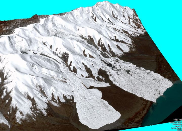
Three dimensional CNES Pléiades image of the avalanches. Processed by Etienne Berthier. Via Twitter.
This article was published by NASA’s Jet Propulsion Laboratory on January 23, 2018. NASA is beginning several months of commemoration of the beginning of the Space Age and the evolution of Earth science from space.
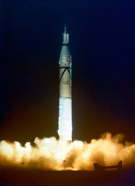
Sixty years ago next week, the hopes of Cold War America soared into the night sky as a rocket lofted skyward above Cape Canaveral, a soon-to-be-famous barrier island off the Florida coast.
The date was Jan. 31, 1958. NASA had yet to be formed, and the honor of this first flight belonged to the U.S. Army. The rocket’s sole payload was a javelin-shaped satellite built by the Jet Propulsion Laboratory in Pasadena, California. Explorer 1, as it would soon come to be called, was America’s first satellite.

“The launch of Explorer 1 marked the beginning of U.S. spaceflight, as well as the scientific exploration of space, which led to a series of bold missions that have opened humanity’s eyes to new wonders of the solar system,” said Michael Watkins, current director of JPL. “It was a watershed moment for the nation that also defined who we are at JPL.”
In the mid-1950s, both the United States and the Soviet Union were proceeding toward the capability to put a spacecraft in orbit. Yet great uncertainty hung over the pursuit. As the Cold War between the two countries deepened, it had not yet been determined whether the sovereignty of a nation’s borders extended upward into space. Accordingly, then-President Eisenhower sought to ensure that the first American satellites were not perceived to be military or national security assets.
In 1954, an international council of scientists called for artificial satellites to be orbited as part of a worldwide science program called the International Geophysical Year (IGY), set to take place from July 1957 to December 1958. Both the American and Soviet governments seized on the idea, announcing they would launch spacecraft as part of the effort. Soon, a competition began between the Army, Air Force and Navy to develop a U.S. satellite and launch vehicle capable of reaching orbit.
At that time, JPL, which was part of the California Institute of Technology in Pasadena, primarily performed defense work for the Army. (The “jet” in JPL’s name traces back to rocket motors used to provide “jet assisted” takeoff for Army planes during World War II.) In 1954, the laboratory’s engineers began working with the Army Ballistic Missile Agency in Alabama on a project called “Orbiter.” The Army team included Wernher von Braun (who would later design NASA’s Saturn V rocket) and his team of engineers. Their work centered around the Redstone Jupiter-C rocket, which was derived from the V-2 missile Germany had used against Britain during the war.
JPL’s role was to prepare the three upper stages for the launch vehicle, which included the satellite itself. These used solid rocket motors the laboratory had developed for the Army’s Sergeant guided missile. JPL would also be responsible for receiving and transmitting the orbiting spacecraft’s communications. In addition to JPL’s involvement in the Orbiter program, the laboratory’s then-director, William Pickering, chaired the science committee on satellite tracking for the U.S. launch effort overall.
The Navy’s entry, called Vanguard, had a competitive edge in that it was not derived from a ballistic missile program — its rocket was designed, from the ground up, for civilian scientific purposes. The Army’s Jupiter-C rocket had made its first successful suborbital flight in 1956, so Army commanders were confident they could be ready to launch a satellite fairly quickly. Nevertheless, the Navy’s program was chosen to launch a satellite for the IGY.
University of Iowa physicist James Van Allen, whose instrument proposal had been chosen for the Vanguard satellite, was concerned about development issues on the project. Thus, he made sure his scientific instrument payload — a cosmic ray detector — would fit either launch vehicle. Meanwhile, although their project was officially mothballed, JPL engineers used a pre-existing rocket casing to quietly build a flight-worthy satellite, just in case it might be needed.
The world changed on Oct. 4, 1957, when the Soviet Union launched a 23-inch (58-centimeter) metal sphere called Sputnik. With that singular event, the space age had begun. The launch resolved a key diplomatic uncertainty about the future of spaceflight, establishing the right to orbit above any territory on the globe. The Russians quickly followed up their first launch with a second Sputnik just a month later. Under pressure to mount a U.S. response, the Eisenhower administration decided a scheduled test flight of the Vanguard rocket, already being planned in support of the IGY, would fit the bill. But when the Vanguard rocket was, embarrassingly, destroyed during the launch attempt on Dec. 6, the administration turned to the Army’s program to save the country’s reputation as a technological leader.
Unbeknownst to JPL, von Braun and his team had also been developing their own satellite, but after some consideration, the Army decided that JPL would still provide the spacecraft. The result of that fateful decision was that JPL’s focus shifted permanently — from rockets to what sits on top of them.
The Army team had its orders to be ready for launch within 90 days. Thanks to its advance preparation, 84 days later, its satellite stood on the launch pad at Cape Canaveral Air Force Station in Florida.
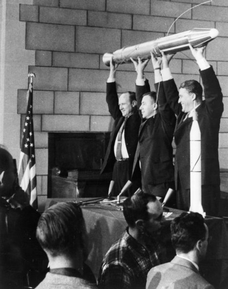
The spacecraft was launched at 10:48 p.m. EST on Friday, Jan. 31, 1958. An hour and a half later, a JPL tracking station in California picked up its signal transmitted from orbit. In keeping with the desire to portray the launch as the fulfillment of the U.S. commitment under the International Geophysical Year, the announcement of its success was made early the next morning at the National Academy of Sciences in Washington, with Pickering, Van Allen and von Braun on hand to answer questions from the media.
Following the launch, the spacecraft was given its official name, Explorer 1. (In the following decades, nearly a hundred spacecraft would be given the designation “Explorer.”) The satellite continued to transmit data for about four months, until its batteries were exhausted, and it ceased operating on May 23, 1958.
Later that year, when the National Aeronautics and Space Administration (NASA) was established by Congress, Pickering and Caltech worked to shift JPL away from its defense work to become part of the new agency. JPL remains a division of Caltech, which manages the laboratory for NASA.
The beginnings of U.S. space exploration were not without setbacks — of the first five Explorer satellites, two failed to reach orbit. But the three that made it gave the world the first scientific discovery in space — the Van Allen radiation belts. These doughnut-shaped regions of high-energy particles, held in place by Earth’s magnetic field, may have been important in making Earth habitable for life. Explorer 1, with Van Allen’s cosmic ray detector on board, was the first to detect this phenomenon, which is still being studied today.
In advocating for a civilian space agency before Congress after the launch of Explorer 1, Pickering drew on Van Allen’s discovery, stating, “Dr. Van Allen has given us some completely new information about the radiation present in outer space….This is a rather dramatic example of a quite simple scientific experiment which was our first step out into space.”
Explorer 1 re-entered Earth’s atmosphere and burned up on March 31, 1970, after more than 58,000 orbits.
For more information about Explorer 1 and the 60 years of U.S. space exploration that have followed it, visit:
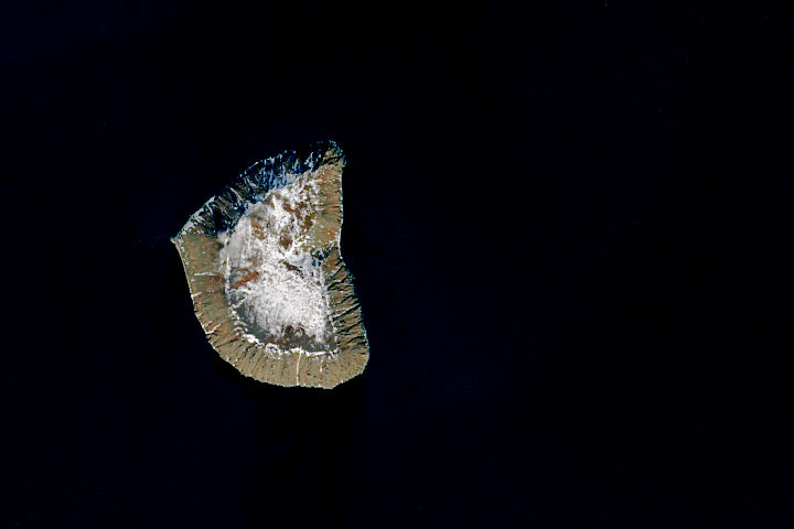
Every month on Earth Matters, we offer a puzzling satellite image. The January 2018 puzzler is above. Your challenge is to use the comments section to tell us what we are looking at, when the image was acquired, and why the scene is interesting.
How to answer. You can use a few words or several paragraphs. You might simply tell us the location. Or you can dig deeper and explain what satellite and instrument produced the image, what spectral bands were used to create it, or what is compelling about some obscure feature in the image. If you think something is interesting or noteworthy, tell us about it.
The prize. We can’t offer prize money or a trip to Mars, but we can promise you credit and glory. Well, maybe just credit. Roughly one week after a puzzler image appears on this blog, we will post an annotated and captioned version as our Image of the Day. After we post the answer, we will acknowledge the first person to correctly identify the image at the bottom of this blog post. We also may recognize readers who offer the most interesting tidbits of information about the geological, meteorological, or human processes that have shaped the landscape. Please include your preferred name or alias with your comment. If you work for or attend an institution that you would like to recognize, please mention that as well.
Recent winners. If you’ve won the puzzler in the past few months or if you work in geospatial imaging, please hold your answer for at least a day to give less experienced readers a chance to play.
Releasing Comments. Savvy readers have solved some puzzlers after a few minutes. To give more people a chance to play, we may wait between 24 to 48 hours before posting comments.
Good luck!
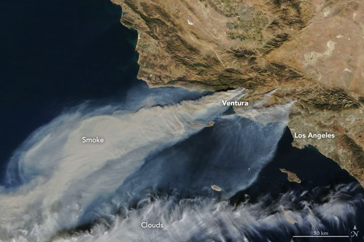
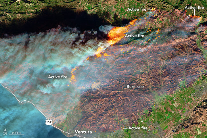
NASA Earth Observatory image by Joshua Stevens, using MODIS data from LANCE/EOSDIS Rapid Response.
With thousands of homes threatened by intense wildfires burning in southern California, NASA Earth Observatory checked in with Jet Propulsion Laboratory scientist Natasha Stavros to learn more about the destructive blazes.
Earth Observatory (EO): Why have these fires been so fast-moving and destructive? Are fierce Santa Ana winds the key factor? Are anomalous temperatures, rainfall, ENSO conditions, bark beetle activity, or other factors playing an important role?
There are absolutely other factors. Santa Ana winds definitely played a role in spreading the fires, but the late fire season is a more complex story. Last year, we had a lot of heavy rains, and this increased fuel connectivity by enabling grasses and annual shrubs to flourish (hence the green hills last spring). However, we had a lot of record-breaking heat waves this year.
In fact, a recent study we conducted with NASA DEVELOP and the National Park Service in the Santa Monica Mountains showed that the number of days over 95 degrees Fahrenheit stressed established vegetation and contributed to massive die-off. Even though the drought is over, the trees are still recovering from the stress of reduced water availability for such an extended period. They are in a fragile state and their defenses are down. This means that they are even more susceptible to infestation, mortality, and ultimately fire danger.
EO: We have published MODIS (top of the page), Sentinel-2 (below), and nighttime VIIRS (bottom of the page) satellite imagery of these fires. Is there anything that you find particularly interesting or notable about these images?
To me, the noteworthy thing is that the plume is going over the ocean and not the continental United States (as we saw earlier this year). This has to do with the Santa Ana winds coming from the desert and pushing particulates, ozone, carbon monoxide, and other toxic pollutants away from where people live.
NASA Earth Observatory image by Joshua Stevens, using modified Copernicus Sentinel data (2017) processed by the European Space Agency.
As for the Sentinel-2 image, this is a great shot in that it really shows the value of remote sensing in monitoring fire. Flames that look like that are tens of meters tall. The flame length is proportional to the heat released from the flame, so these fires are very hot. Just like you would not want to stand too close to a bonfire with flames tens of meters tall, fire management does not want to put personnel in the path of those flames.
Images like these and fire behavior models help inform how we think the fire will move across the landscape. There is still a lot we do not know; our models are based on what we do know, so as fires become more intense, the models do not work as well, so this is an area of active research.
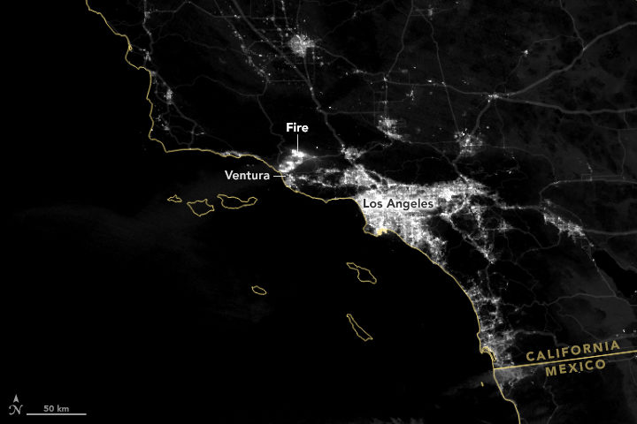
NASA Earth Observatory images by Joshua Stevens using VIIRS day-night band data from the Suomi National Polar-orbiting Partnership.
EO: Is there anything to say about how these fires fit into longer term trends and/or changing climate patterns?
Fire regimes are changing. There is no question about that, and there are a lot of things contributing to it: climate change, a century of fire exclusion, and a growing wildland urban interface (WUI). As we move into the future, we expect there to be an increase in very large fire events. Also, and this is relevant for the events happening now, there will be longer fire seasons. Also, note that many of the fires that ignite close to where people live are actually caused by people. This is particularly true in Southern California.
As we move forward, we need to think about how to support smart fire management practices. By that I mean: what can we proactively do to reduce fire risk (i.e. the threat to valuable resources)?
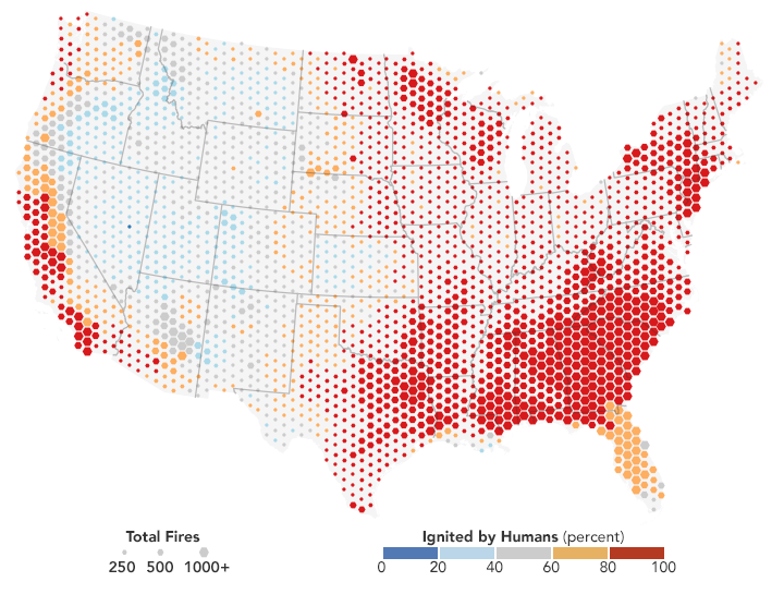
Most fires on the coasts are lit by people. NASA Earth Observatory map by Joshua Stevens, using fire data courtesy of Balch, J. et al. (2017).
EO: What about JPL’s response to these fires? I was intrigued by the megafire project described here. Will your group be responding to this fire in any way?
We just received approval from NASA Headquarters to fly the Airborne Visible/Infrared Imaging Spectrometer (AVIRIS) over these fires. This sensor has been useful for investigating fuel load type and subsequent effects on emission types, fire behavior, and post-fire analysis (e.g., safety, erosion, area burned, fire severity or the amount of environmental change caused the fire, etc.) and is often analyzed in interagency and federal-academic coordination to improve our understanding of fire.
Another effort to support fire management includes work being done from JPL in coordination with the National Interagency Fire Center (NIFC) to help them develop metrics of fire danger using NASA satellites that provide hydrologic variables (e.g., soil moisture and vapor pressure deficit—the difference between the amount of moisture in the air vs how much it can hold). These metrics have a one-month forecast to help allocate fire management resources nationally, which is particularly important as our fire seasons extend throughout the year in multiple places at the same time.

Natasha Stavros. Image courtesy of N. Stavros.
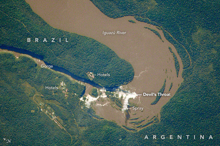
In 2016, we published space-based imagery of Iguazú Falls—South America’s famous system of waterfalls, which is near a bend in the Iguazú River between Argentina and Brazil. Spray from the falls reaches so high that it is visible from space. A crew member aboard the International Space Station captured the photograph above on May 24, 2016.
The view from the ground is also quite compelling, attracting more than a million visitors per year. The images below show ground-based views of the falls, photographed photographed by NASA’s Alexey Chibisov from the Argentine side of the river on November 28, 2017. Chibisov took the photos while on vacation after weeks in the field with the Operation IceBridge mission.
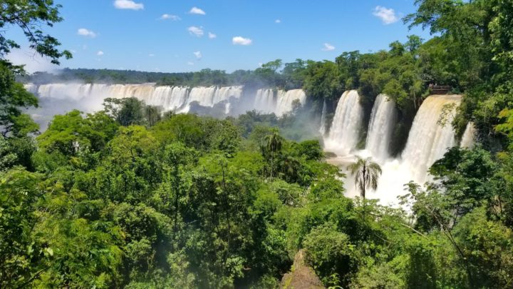
Photo by Alexey Chibisov.
Lush, subtropical rainforest surrounds the falls. The vegetation here is part of a remaining fragment of the Atlantic Forest, which stretches from the east coast of South America inland toward the Amazon. The forest is habitat for tens of thousands of plant species and thousands of animal species.
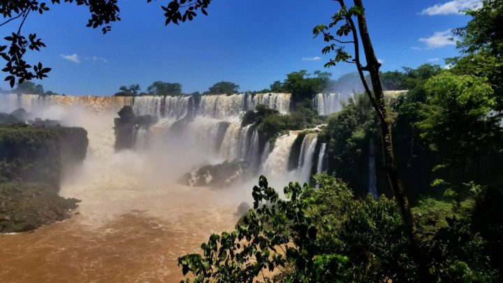
Photo by Alexey Chibisov.
Sediment carried by the fast-moving river can impart a red-brown color to the water, especially after periods of heavy rain.
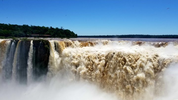
Photo by Alexey Chibisov.
The mist is the result of water that plunges as much as 260 feet (80 meters) over layers of basalt cliffs.

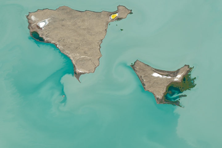
Every month on Earth Matters, we offer a puzzling satellite image. The November 2017 puzzler is above. Your challenge is to use the comments section to tell us what we are looking at, when the image was acquired, and why the scene is interesting.
How to answer. You can use a few words or several paragraphs. You might simply tell us the location. Or you can dig deeper and explain what satellite and instrument produced the image, what spectral bands were used to create it, or what is compelling about some obscure feature in the image. If you think something is interesting or noteworthy, tell us about it.
The prize. We can’t offer prize money or a trip to Mars, but we can promise you credit and glory. Well, maybe just credit. Roughly one week after a puzzler image appears on this blog, we will post an annotated and captioned version as our Image of the Day. After we post the answer, we will acknowledge the first person to correctly identify the image at the bottom of this blog post. We also may recognize readers who offer the most interesting tidbits of information about the geological, meteorological, or human processes that have shaped the landscape. Please include your preferred name or alias with your comment. If you work for or attend an institution that you would like to recognize, please mention that as well.
Recent winners. If you’ve won the puzzler in the past few months or if you work in geospatial imaging, please hold your answer for at least a day to give less experienced readers a chance to play.
Releasing Comments. Savvy readers have solved some puzzlers after a few minutes. To give more people a chance to play, we may wait between 24 to 48 hours before posting comments.
Good luck!
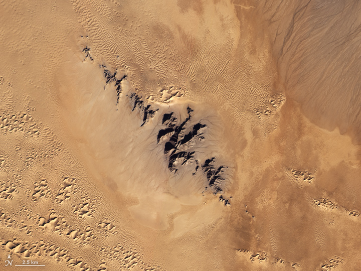
In this satellite image, the prominent Pinacate Peaks stick out above the sand dune landscape of the Gran Desierto de Altar in Mexico’s Sonoran Province. The peaks are located just south of the Mexico-United States border. The Gran Desierto de Altar is one section of the broader Soronan Desert which covers much of northwestern Mexico and reaches into Arizona and California.
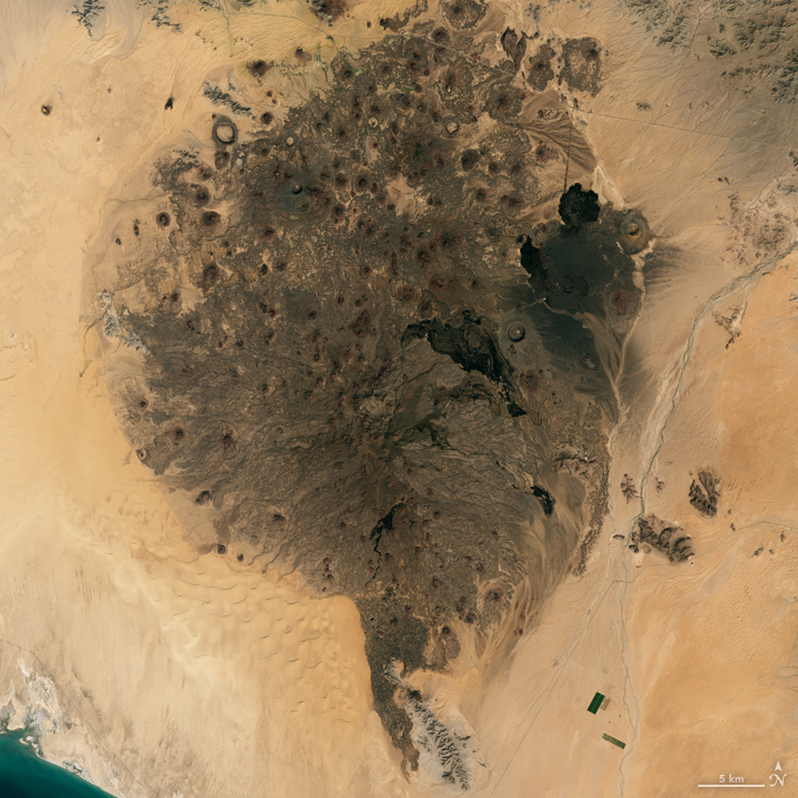
Steady, consistent winds in the area have shifted low-lying sand into dune fields in intriguing regular patterns. These same patterns of sand dune fields appear around the world in desert areas.
The volcanic peaks and cinder cones are believed to have formed from volcanic activity that first started roughly 4 million years ago — most likely due to the plate tectonics that also formed the Gulf of California around the same time. The most recent activity was perhaps 11,000 years ago. During the late 1960s, NASA trained astronauts in field geology at a number of sites around the world, including Pinacate Peaks, as preparation for the lunar landings.
The natural color image here is from the Landsat 8 satellite using its Operational Line Imager (OLI) instrument. The image was acquired on October 3, 2017. The volcanic cinder cone field stains the landscape of bright sand and tall dunes in the El Pinacate y Gran Desierto de Altar Biosphere Reserve.
NOTE: In a previous version of this post, I featured the EO-1 ALI image below, and an astute reader pointed out that these peaks, while in the Biosphere Reserve, are not Pinacate Peaks, but rather the Sierra de Rosario range nearby. I am geographically and tectonically embarassed…
The natural color image here is from the now-defunct Earth Observing 1 (EO-1) satellite using its Advanced Land Imager (ALI). The image was acquired on December 16, 2012. This late-year scene was just days before the solstice (the farthest south the Sun appears in the sky), so the tallest sand dunes and the volcanic peaks cast unusually long shadows across the ground.
EO-1 was launched in November 2000 as an engineering testbed for new sensor technology; in particular, the ALI instrument was a predecessor for the Landsat 8 Operational Land Imager. The EO-1 mission was so successful that it was extended past its original 18-month mission, and was only recently retired after 17 years of operation.
This post is republished from the Landsat science team page.
In the giddy, early days following the flawless launch of Landsat 8, as the satellite commissioning was taking place, the calibration team noticed something strange. Light and dark stripes were showing up in images acquired by the satellite’s Thermal Infrared Sensor (TIRS).
Comparing coincident data collected by Landsat 8 and Landsat 7 — acquired as Landsat 8 flew under Landsat 7, on its way to its final orbit — showed that thermal data collected by Landsat 8 was off by several degrees.

This was a big deal. The TIRS sensor had been added to the Landsat 8 payload specifically because it had been deemed essential to a number of applications, especially water management in the U.S’s arid western states.
The TIRS error source was a mystery. The prelaunch TIRS testing in the lab had shown highly accurate data (to within 1 degree K); and on-orbit internal calibration measurements (measurements taken of an onboard light source with a known temperature) were just as good as they had been in the lab. But when TIRS radiance measurements were compared to ground-based measurements, errors were undeniably present. Everywhere TIRS was reporting temperatures that were warmer than they should have been, with the error at its worst in regions with extreme temperatures like Antarctica.
After a year-long investigation, the TIRS team found the problem. Stray light from outside the TIRS field-of-view was contaminating the image. The stray light was adding signal to the TIRS images that should not have been there—a “ghost signal” had been found.
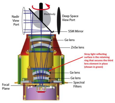
Scans of the Moon, together with ray tracing models created with a spare telescope by the TIRS instrument team, identified the stray light culprit. A metal alloy retaining ring mounted just above the third lens of the four-lens refractive TIRS telescope was bouncing out-of-field reflections onto the TIRS focal plane. The ghost-maker had been found.
With the source of the TIRS ghosts discovered, Matthew Montanaro and Aaron Gerace, two thermal imaging experts from the Rochester Institute of Technology, were tasked with getting rid of them.
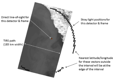
Montanaro and Gerace had to first figure out how much energy or “noise” the ghost signals were adding to the TIRS measurements. To do this, a stray light optical model was created using reverse ray traces for each TIRS detector. This essentially gave Montanaro and Gerace a “map” of ghost signals. Because TIRS has 1,920 detectors, each in a slightly different position, it wasn’t just one ghost signal they had to deal with— it was a gaggle of ghost signals.
To calculate the ghost signal contamination for each detector, they compared TIRS radiance data to a known “correct” top-of-atmosphere radiance value (specifically, MODIS radiance measurements made during the Landsat 8 / Terra underflight period in March 2013).
Comparing the MODIS and TIRS measurements showed how much energy the ghost signal was adding to the TIRS radiance measurements. These actual ghost signal values were then compared to the model-based ghost signal values that Montanaro and Gerace had calculated using their stray light maps and out-of-field radiance values from TIRS interval data (data collected just above and below a given scene along the Landsat 8 orbital track).
Using the relationships established by these comparisons, Montanaro and Gerace came up with generic equations that could be used to calculate the ghost signal for each TIRS detector.
Once the ghost signal value is calculated for each pixel, that value can be subtracted from the measured radiance to get a stray-light corrected radiance, i.e. an accurate radiance. This algorithm has become known as the “TIRS-on-TIRS” correction. After performing this correction, the absolute error can be reduced from roughly 9 K to 1 K and the image banding, that visible vestige of the ghost signal, largely disappears.
“The stray light issue is very complex and it took years of investigation to determine a suitable solution,” Montanaro said.
This work paid off. Their correction—hailed as “innovative” by the Landsat 8 Project Scientist, Jim Irons—has withstood the scrutiny of the Landsat Science Team. And Montanaro and Gerace’s “exorcism” has now placed the Landsat 8 thermal bands in-line with the accuracy of the previous (ghost-free) Landsat thermal instruments.
USGS EROS has now implemented the software fix developed by these “Landsat Ghostbusters” as part of the Landsat Collection 1 data product. Savvy programmers at USGS, led by Tim Beckmann, made it possible to turn the complex de-ghosting calculations into a computationally reasonable fix that can be done for the 700+ scenes collected by Landsat 8 each day.
“EROS was able to streamline the process so that although there are many calculations, the overall additional processing time is negligible for each Landsat scene,” Montanaro explained.

Gerace is now determining if an atmospheric correction based on measurements made by the two TIRS bands, a technique known as a split window atmospheric correction, can be developed with the corrected TIRS data.
Meanwhile, Montanaro has been asked to support the instrument team building the Thermal Infrared Sensor 2 that will fly on Landsat 9. A hardware fix for TIRS-2 is planned. Baffles will be placed within the telescope to block the stray light that haunted the Landsat 8 TIRS.
The Landsat future is looking ghost-free.
Related Reading:
+ RIT University News
+ TIRS Stray Light Correction Implemented in Collection 1 Processing, USGS Landsat Headline
+ Landsat Level-1 Collection 1 Processing, USGS Landsat Update Vol. 11 Issue 1 2017
+ Landsat Data Users Handbook, Appendix A – Known Issues
References:
Montanaro, M., Gerace, A., Lunsford, A., & Reuter, D. (2014). Stray light artifacts in imagery from the Landsat 8 Thermal Infrared Sensor. Remote Sensing, 6(11), 10435-10456. doi:10.3390/rs61110435
Montanaro, M., Gerace, A., & Rohrbach, S. (2015). Toward an operational stray light correction for the Landsat 8 Thermal Infrared Sensor. Applied Optics, 54(13), 3963-3978. doi: 10.1364/AO.54.003963 (https://www.osapublishing.org/ao/abstract.cfm?uri=ao-54-13-3963)
Barsi JA, Schott JR, Hook SJ, Raqueno NG, Markham BL, Radocinski RG. (2014) Landsat-8 Thermal Infrared Sensor (TIRS) Vicarious Radiometric Calibration. Remote Sensing, 6(11), 11607-11626.
Montanaro, M., Levy, R., & Markham, B. (2014). On-orbit radiometric performance of the Landsat 8 Thermal Infrared Sensor. Remote Sensing, 6(12), 11753-11769. doi: 10.3390/rs61211753
Gerace, A., & Montanaro, M. (2017). Derivation and validation of the stray light correction algorithm for the Thermal Infrared Sensor onboard Landsat 8. Remote Sensing of Environment, 191, 246-257. doi: 10.1016/j.rse.2017.01.029
Gerace, A. D., Montanaro, M., Connal, R. (2017). Leveraging intercalibration techniques to support stray-light removal from Landsat 8 Thermal Infrared Sensor data. Journal of Applied Remote Sensing, Accepted for Publication.
Every month on Earth Matters, we offer a puzzling satellite image. The October 2017 puzzler is above. Your challenge is to use the comments section to tell us what we are looking at, when the image was acquired, and why the scene is interesting.
How to answer. Your answer can be a few words or several paragraphs. (Try to keep it shorter than 200 words). You might simply tell us what part of the world an image shows. Or you can dig deeper and explain what satellite and instrument produced the image, what spectral bands were used to create it, or what is compelling about some obscure speck in the far corner of an image. If you think something is interesting or noteworthy, tell us about it.
The prize. We can’t offer prize money or a trip to Mars, but we can promise you credit and glory. Well, maybe just credit. Roughly one week after a puzzler image appears on this blog, we will post an annotated and captioned version as our Image of the Day. After we post the answer, we will acknowledge the person who was first to correctly ID the image at the bottom of this blog post. We may also recognize certain readers who offer the most interesting tidbits of information about the geological, meteorological, or human processes that have played a role in molding the landscape. Please include your preferred name or alias with your comment. If you work for or attend an institution that you want us to recognize, please mention that as well.
Recent winners. If you’ve won the puzzler in the last few months or work in geospatial imaging, please sit on your hands for at least a day to give others a chance to play.
Releasing Comments. Savvy readers have solved some of our puzzlers after only a few minutes or hours. To give more people a chance to play, we may wait between 24-48 hours before posting the answers we receive in the comment thread.
Good luck!
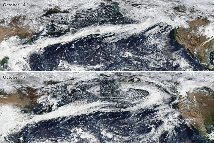
Atmospheric rivers stretched from Asia to North America in October 2017. Learn more.
If you live on the West Coast of North America, you have probably heard meteorologists talk about “atmospheric rivers” — the narrow, low-level plumes of moisture that often accompany extratropical storms and transport large volumes of water vapor across long distances. When atmospheric rivers encounter land, they can drop tremendous amounts of rain and snow. That can be good for replenishing reservoirs and for quenching droughts, but these remarkable meteorological features can also trigger destructive floods, landslides, and wind storms.
During the past decade, atmospheric rivers have fueled a flood of another type: scientific research papers. Prior to 2004, fewer than 10 studies mentioned atmospheric rivers in any given year; in 2015, about 200 studies were published on the matter. The availability of increasingly sophisticated satellite and aircraft data has fueled the trend, according to a recent article in the Bulletin of the American Meteorological Society. Here’s a sampling of what scientists have learned about these rivers in the sky.
They Can Bring Rains, Winds, And Lots of Damage
In a study led by Duane Waliser of NASA’s Jet Propulsion Laboratory and published in Nature Geoscience, researchers showed that atmospheric rivers are among the most damaging storm types in the middle latitudes. Of the wettest and windiest storms (those ranked in the top 2 percent), atmospheric rivers were associated with nearly half of them. Waliser and colleagues found that atmospheric rivers were associated with a doubling of wind speed compared to all storm conditions.
They Shift With The Seasons
During the winter, atmospheric rivers in the Pacific generally shift northward and westward, Bryan Mundhenk of Colorado State University and colleagues concluded in a study. They also found that the El Niño/Southern Oscillation (ENSO) cycle can affect the frequency of atmospheric river events and shift where they occur. The research was based on data processed by MERRA, a NASA reanalysis of meteorological data from satellites.
They Aren’t Just a West Coast Thing
Atmospheric rivers are a global phenomenon and responsible for about 22 percent of all water runoff. One recent study from a University of Georgia team underscored that the U.S. Southeast sees a steady stream of atmospheric rivers. “They are more common than we thought in the Southeast, and it is important to properly understand their contributions to rainfall given our dependence on agriculture and the hazards excessive rainfall can pose,” said Marshall Shepherd of the University of Georgia. Other studies note that atmospheric rivers have contributed to anomalous snow accumulation in East Antarctica and extreme rainfall in the Bay of Bengal.
Climate Change Could Alter Them
A recent study led by Christine Shields of the National Center for Atmospheric Research suggests that climate change could push atmospheric rivers in the Pacific toward the equator and bring more intense rains to southern California. The modeling calls for smaller increases in rain rates in the Pacific Northwest. Another ensemble of models shows a in the number of days with landfalling atmospheric rivers in western North America.
Satellites Are Key to Studying Their Precipitation
While there are few ground-based weather stations in the open ocean to tally how much rain falls, satellites such as those included in the Global Precipitation Measurement (GPM) mission can estimate precipitation rates from above. “Satellites have proven valuable over both the ocean and land, though uncertainties are often larger over land because of complicating factors like the terrain and the presence of snow on the surface,” said Ali Behrangi, the author of a study that assessed the skill of different satellite-derived measurements of precipitation rates.
