A Powerful Landscape
Umbrella in one hand, I gripped the metal cable of the suspension bridge as I looked down into the boiling Bhotekosi River coursing below me through a steep, verdant canyon. Due to the steep slopes, fragile geology, and frequent rainfall, Nepal is especially subject to natural disasters including landslides and flooding.
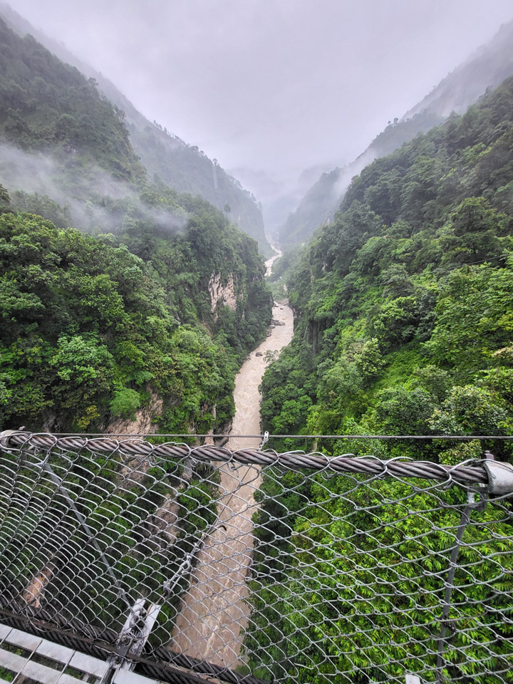
I found myself in this powerful landscape because I work for SERVIR, a joint NASA and USAID program that works with leading regional organizations to help countries worldwide use Earth observations and geospatial technologies to address environmental challenges. I joined a group of scientists and disaster risk reduction practitioners on a trip to view major landslide sites and better understand what satellite data can tell us about the landscape. Driving up from Kathmandu, we passed by small villages, hydropower plants, bulging retaining walls holding back hillsides, and the aftermath of past destructive landslides.
As an applied remote sensing scientist, I seek to understand the physical processes driving these hazards, how satellite data can capture these processes, and how the information from satellite data can complement the existing systems used for planning, early warning, and disaster response. While satellite data has the distinct advantage of consistently receiving data over large regions of the world, it is only a single perspective.
Visiting the field, talking to experts, and consulting with end users is critical to designing a product that is effective at reducing loss of lives and infrastructure due to natural hazards.
Cascading Hazards in Nepal
Cascading hazards (or ‘multi-hazards’) are events where one hazard triggers or increases vulnerability of a second hazard, such as a landslide that blocks a river and creates a flood. They pose a challenge to disaster managers since they can evolve quickly and the outcome can be difficult to predict. Nepal’s predominantly rural population is increasingly at risk as climate change drives extreme and erratic precipitation events that trigger cascading hazards.
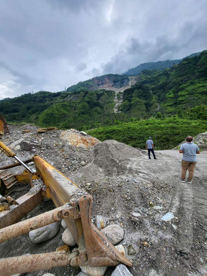
During our drive, we stopped to look at the site of the Jure landslide on the right bank of the Sunkoshi River. In 2014, the Jure landslide broke free from the steep valley walls, plummeting thousands of meters to the valley floor, blocking the river, and destroying over 100 homes and lives. The natural dam quickly caused water to back up, posing a serious flood risk to upstream towns and damaging hydropower infrastructure. The Nepal Army and Police force acted quickly to dynamite a section of the dam to release some of the water downstream, but even after this quick action the threat of catastrophic flood remained. Fortunately, a month later when the dam breached, no major damage was caused by the flood waters. In addition to loss of lives and homes, damage to the road interrupted necessary services, disrupted the primary trade route with China, and impacted the tourism trade.
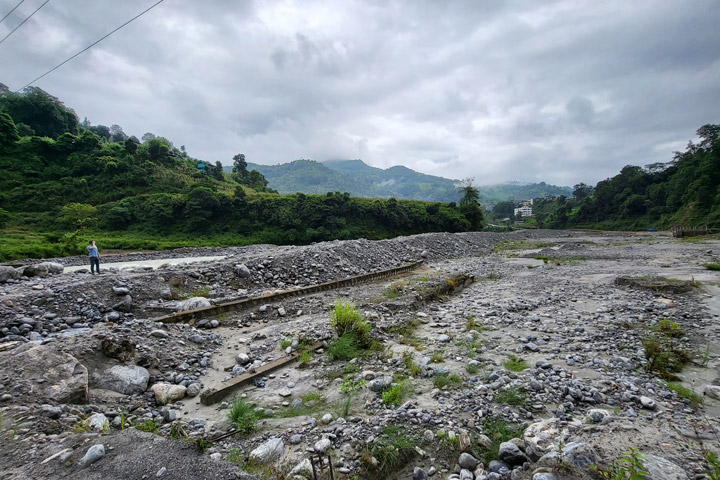
In addition to precipitation events, several factors increase the chance of cascading hazards in this region: glacial lakes, snowmelt, permafrost degradation, glacial deposits, high relief, and fragile topography. The Melamchi flood disaster that occurred June 15th of 2021 was triggered by heavy rainfall at higher elevations and snowmelt. This increased amount of drainage caused a glacial lake to breach. The consequent erosion of glacial deposits and natural dams downstream resulted in severe flooding that carried debris the size of boulders and triggered further landslides and riverbank erosion.
The communities here are familiar with the risk of natural hazards. They know that there is a higher risk of landslides when it rains. The current mechanisms for warning are primarily word of mouth, phone calls, text messages, and social media posts. Despite these warnings, many lives are lost during these disasters. There is still a need for an integrated multi-hazard early warning system.
The Satellite Perspective
Satellite data can be used to consistently monitor large areas for potential hazards, such as slopes at risk for landslides. Factors such as precipitation, soil moisture, slope, aspect, and even slow-motion movement can be measured via satellite and contribute to landslide hazard mapping.
NASA’s High Mountain Asia Team (HiMAT) is a group of scientists focusing on bringing the satellite perspective to these hazards. Thomas Stanley and Pukar Amatya from UMBC/NASA worked together with Sudan Bikash Maharjan from International Center for Integrated Mountain Development (ICIMOD) to develop a prototype landslide mapping and hazard awareness tool for the Karnali River Basin in Nepal. Collaborating with the National Disaster Risk Reduction and Management Authority (NDRRMA) and other government agencies, they are working to integrate the landslide hazard awareness tool into the planning and early warning process. In addition, a SERVIR applied science team is looking at how satellite radar systems can be used to monitor slowly moving slopes in the region.
The hazard awareness tool is known as Landslide Hazard Awareness for Karnali (LHASKarnali). It is a pilot project to adapt the global Landslide Hazard Assessment for Situational Awareness (LHASA) model for use in High Mountain Asia starting with the Karnali River Basin of Nepal. LHASA was previously regionalized for a SERVIR Applied Science Team project in the Lower Mekong region. It provides a one-day forecast of the hazard level for rainfall-triggered landslides by using precipitation forecasts. The LHASKarnali tool integrates forecasted precipitation from the High-Impact Weather Assessment Toolkit (HiWAT), which is managed by ICIMOD.
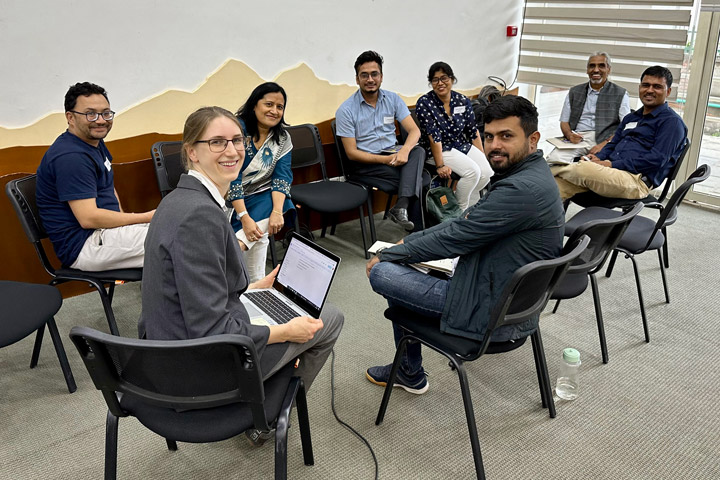
At a workshop prior to our field visit, we sought the insights of national stakeholders and academic experts, including the Department of Mines and Geology and the Department of Hydrology and Meteorology. Drawing from their experience assessing slope stability for high-risk communities, they felt that soil depth and soil moisture were among the most important factors controlling the occurrence of rain-triggered landslides. While satellite data can accurately provide data on slope, aspect, and rainfall, soil moisture is not well captured due to the steep slopes and high vegetation cover in Nepal. Although prior rainfall was used in LHASKarnali as a proxy for soil moisture, how this translates to soil moisture is unknown. These conversations helped end users think through the value of the tool and how their expertise could be used to enhance the end-product going forward.
The limitations of a 4-kilometer resolution product also stood out to participants. Response agencies like Practical Action emphasized the need to be able to identify vulnerable populations at a household or village level. Even smaller landslides can be highly destructive and more targeted warnings are important when evacuations and other high effort actions are required. Going forward, a partnership between the scientists and universities will contribute to an effort to increase the resolution of the landslide hazard forecast.
Looking Ahead
During my time in Nepal, I traversed steep river canyons, which showed me the challenge of capturing and interpreting the steep slopes and narrow rivers in satellite imagery. Talking with disaster management agencies like Practical Action and NDRRMA, I learned about the need for a joint system for multi-hazard assessment to understand the cumulative effects of landslides, floods, and other factors like the erosion of natural dams. Getting the opportunity to speak with communities and get feedback about satellite observations, such as concerns over the representation of soil moisture, help us get closer to achieving warning systems for these complex hazards.
With increasing extreme events due to climate change, being able to plan and react to these hazards is critical for resilience. It will take collective expertise and tools to tackle this complex challenge.
Fieldwork notes, July 21-August 3, 2023
Summer fieldwork for our project, “Clarifying Linkages Between Canopy Solar Induced Fluorescence (SIF) and Physiological Function for High Latitude Vegetation,” once again took our team from University of Maryland Baltimore County north to the boreal forests of central Alaska. We visited this area in the spring to collect data during the very start of the growing season, and now we are returning to collect data during the peak of summer.
This project is part of the NASA Terrestrial Ecology program’s Arctic-Boreal Vulnerability Experiment (ABoVE). The goal of ABoVE is to improve our understanding of high latitude ecosystems, how these ecosystems respond to climate change, and how satellite data can provide information to describe ecosystem processes and aid management decisions.
Our study focuses on measuring light emitted by plants called solar induced fluorescence. Green leaves absorb light, and through photosynthesis take in carbon dioxide and water and produce oxygen and sugars. Fluorescence occurs during photosynthesis as some of the absorbed light energy is radiated out from the plant. The amount of light fluoresced is only a very small fraction of what is absorbed, which is why our eyes don’t see plants glowing. In our study, we use sensitive instruments that can detect this fluorescence. Our goal is to better understand the sources of fluoresced light and how to use this information to describe productivity in boreal forests and tundra.
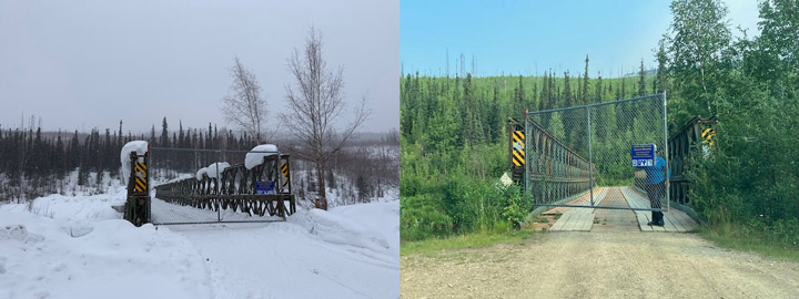
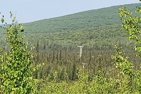
Our study site is at the Caribou Creek flux tower run by the National Science Foundation’s National Ecological Observatory Network (NEON). In spring, we deployed automated instruments at the NEON tower site that continuously collect data. On this trip, we are checking on how they have been working.
In July there was a big change from our previous visit in April. In April, the area had a deep snow cover with temperatures dropping below 0°F, while during this visit the daytime temperatures were in the 80s F and the ground was now all green (images below).
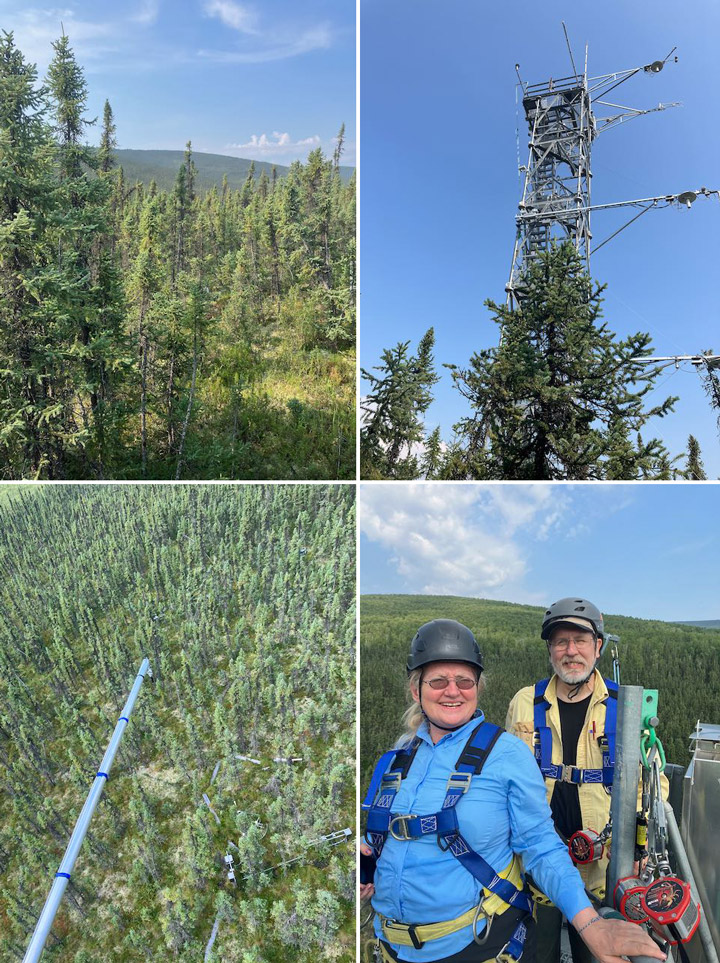
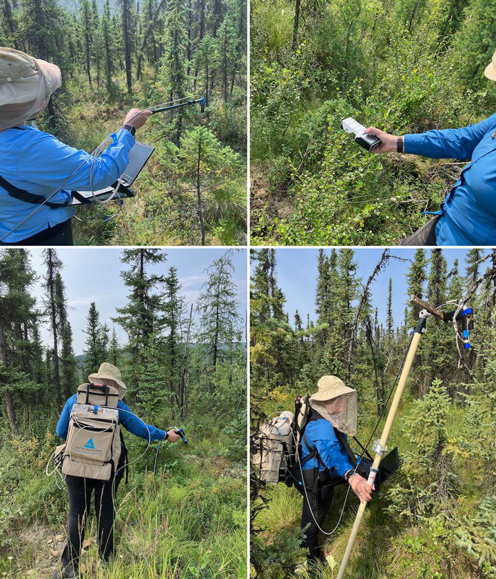
On the top of the tower we have an instrument called a FLoX (Fluorescence Box). The FLoX views a patch of forest from above, and every few minutes during the day it measures the reflected light and solar induced chlorophyll fluorescence. This provides us with a description of plant activity at different times of the day through the growing season (images below).
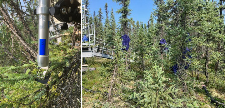
Also at the site we have monitoring PAM (MoniPAM) instruments attached to shoots of the spruce trees. The MoniPAM probes shine pulses of light at individual spruce shoots to measure fluorescence and photosynthetic processes at the leaf level (images below). We put blankets over the probes for a while to dark-adapt the shoots to measure their response when unstressed. In the spring, we put the MoniPAM probes in easy-to-reach places when there was a lot of snow on the ground. On this trip, when we returned to check them in the summer, we found we had to really reach up to get them without the snow to stand on.
From the ground, we collected reflectance and fluorescence measurements (similar to the data collected by the FLoX) of individual plants in the FLoX field of view and a variety of representative plants in the larger area surrounding the tower. These measurements will help us understand the local variability (images below).
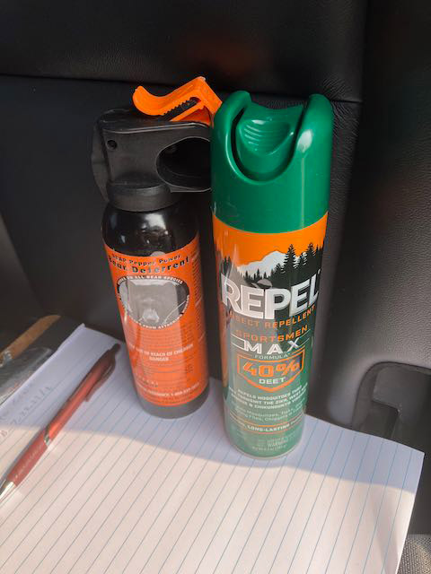
A lot of the ground cover was cotton grass (Eriophorum spp.) that forms tussocks, which are tight clumps of grasses. The tussocks made walking through the area difficult, like walking on half-buried basketballs, so it was easy to twist an ankle, especially with a heavy backpack spectrometer on your back.
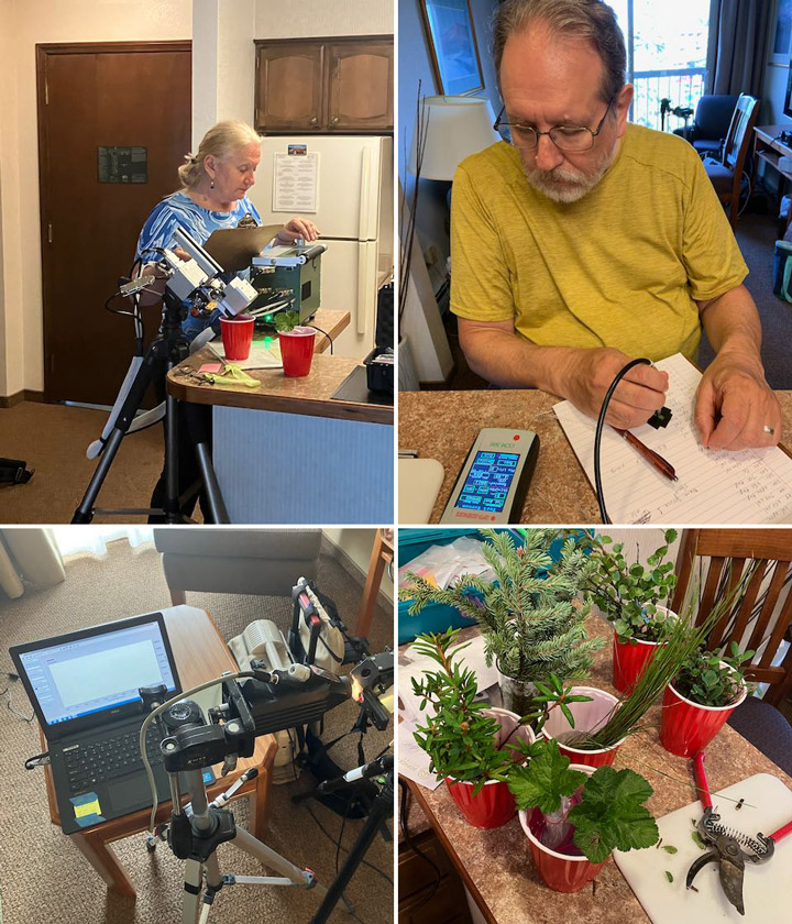
We collected branch samples to make measurements of leaves and needles that we will use to parameterize models of vegetation fluorescence and productivity (images below).
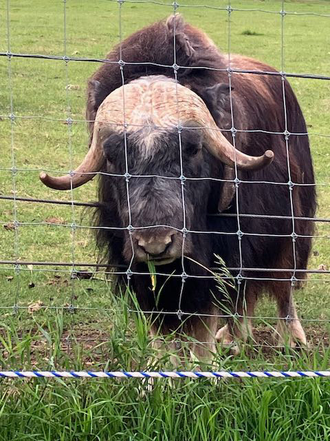
We took a little time off to visit some other places in the area. We saw musk ox, which are animals of the tundra but raised in captivity at the University of Alaska Fairbanks’ Large Animal Research Station. Their thick, shaggy coat keeps them warm through the frigid arctic winters. Under the long guard hairs is a soft wool called qiviut that musk oxen shed in the spring. Qiviut can be spun into a very warm and soft yarn. Small balls of qiviut yarn can sell for over $100.
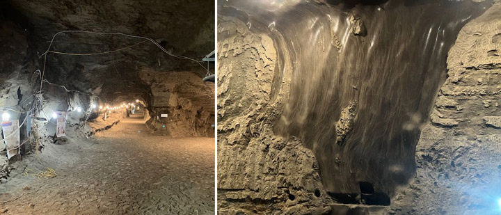
On our last day in Alaska we visited the Cold Regions Research and Engineering Laboratory (CRREL) Permafrost Tunnel Research Facility (images below). Permafrost refers to soil that has been frozen continuously for more than two years. The permafrost around Fairbanks, Alaska, is considered ‘warm’ (at a temperature of -0.3oC/-0.4oC) as compared to the permafrost in our other study site in the North Slope of Alaska at Utqiagvik (e.g., a temperature -3oC/-4 oC). This warm permafrost is very sensitive to the changes in soil temperatures that can result from fires, rain events, and other disruptions that can cause permafrost thawing. Thawing permafrost can result in damage to roads and buildings and cause disturbance in forests.
The permafrost tunnel is dug into a hillside through earth that has been frozen for thousands of years. The tunnel reveals bones of extinct ice age animals, plants preserved since the ice age, and large ice wedges that can take hundreds to thousands of years to form. The ice wedges cause the formation of polygonal patterned ground, where the ground surface is covered with a pattern of shapes of slightly higher or lower ground. Our study site in Utqiagvik was in an area of high centered polygons, so it was interesting to be able to actually see the shapes of the underground ice that formed that unique landscape.
In 2022, severe lightning ignited many fires in Alaska. Notably, several exceptionally large fires burned in the tundra of Southwest Alaska, an ecosystem that is traditionally less prone to fire. While our understanding of the carbon emissions of boreal forest fires in Alaska and Canada has strongly advanced in recent years thanks to the work of several teams within NASA’s Arctic-boreal Vulnerability Experiment (ABoVE), the impacts of these tundra fires on the ecosystem’s carbon balance and permafrost has remained less well known.
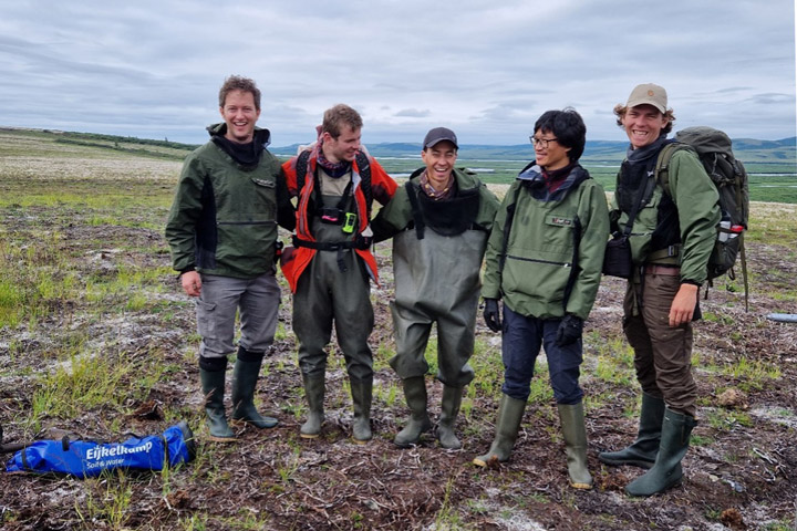
Our Climate and Ecosystems Change research group from the Vrije Universiteit Amsterdam in the Netherlands is currently in Southwest Alaska to fill these critical knowledge gaps. Our team received tremendous help of Dr. Lisa Saperstein from the Alaska Fish and Wildlife Service in organizing the campaign. Lisa will also start a field campaign in the same fires in the next few days and we plan to pool our datasets to maximize synergies between our efforts.
The 2022 East Fork and the Apoon Pass fires together burned more than 100,000 hectares (380 square miles) of primarily tundra landscapes in Southwest Alaska. They were among the largest tundra fires on record for the region.
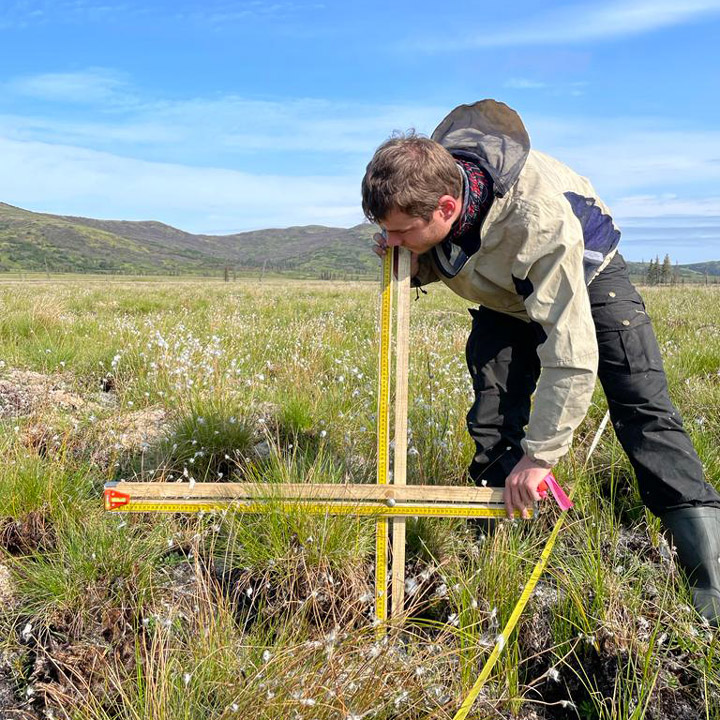
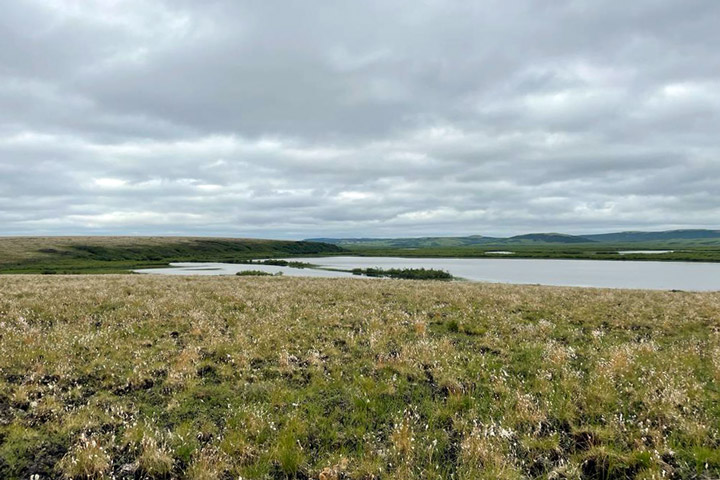
Our basecamp is the village of St. Mary’s, located just west of the East Fork fire on the Andreafsky River. For the first part of our campaign, we are taking a boat upstream to access the fire scar. We are looking for burned tussock tundra sites, where we can measure the effects of the fire on the vegetation, soils, and permafrost in our plots. We are also sampling unburned tundra sites, which provide us a reference of the conditions without fire disturbance. During the last part of our campaign we will access sites in the remote Apoon Pass fire by helicopter.
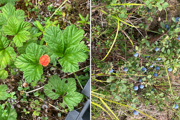
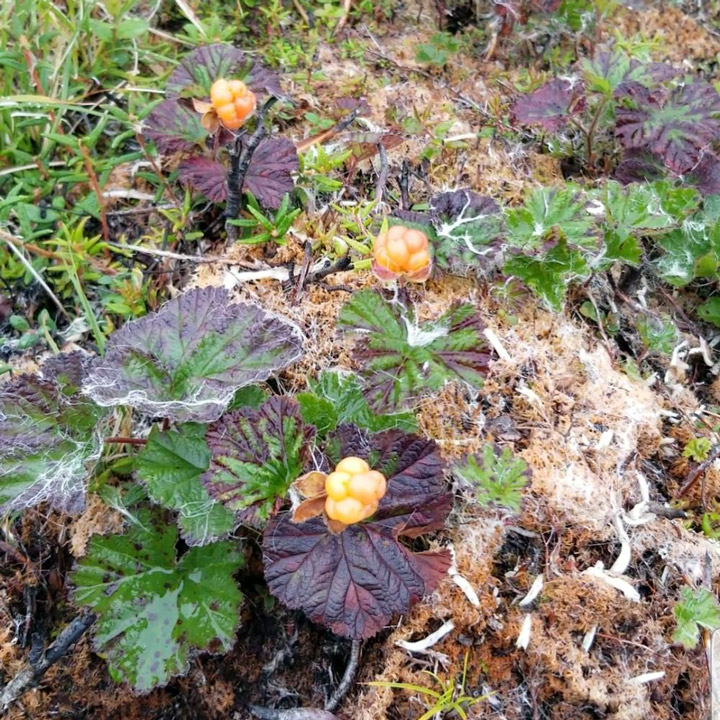
The local community heavily relies on the landscape for subsistence activities, like hunting and berry picking. Our boat driver, Matty Beans, is native to the area and is extremely helpful in bringing us to the right places. A large concern of the community is how the fire has effected the abundance of berries in the burned tundra. Our preliminary observations indicate that the cloudberries, locally also called salmonberries, were abundantly present in the burned sites. However, this was not the case yet for blueberries.
So far, we have been extremely lucky with mostly dry weather and only a little bit of rain. However, the dry weather has affected the water levels in the Andreafsky River. We came across collapsed river banks and exposed sand banks in the river. Our boat driver has switched to his jet boat so that we can continue on, even in more shallow parts of the river. The weather is changing though, with rain coming in for several days. This is good for the water levels, but the colder and rainy weather may make our sampling efforts more challenging.
After seven days and 19 plots of sampling, we are now taking a well-deserved rest day. I used this rest day to write this blog and digitize some datasheets. Over the next four days, we will continue sampling along the river and then use a helicopter to access the Apoon Pass fire site for more sampling.
This field expedition is part of FireIce (Fire in the land of ice: climatic drivers & feedbacks). FireIce is a Consolidator project funded by the European Research Council. FireIce is affiliated with NASA ABoVE.
In loving memory of Larry Corp.
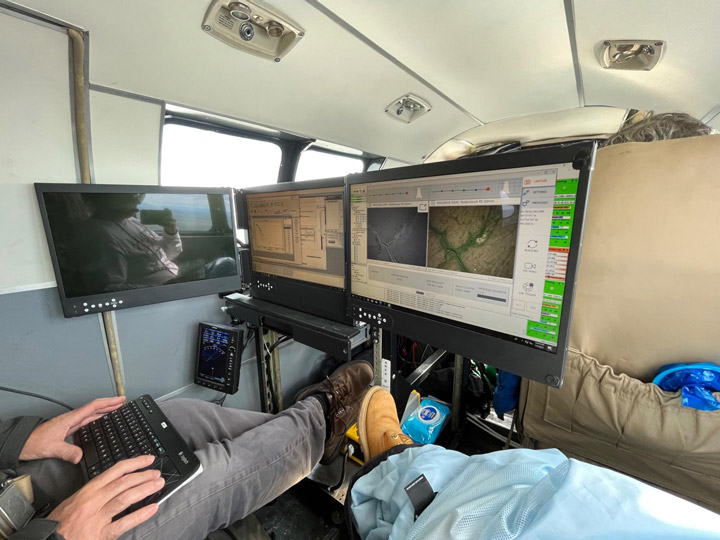
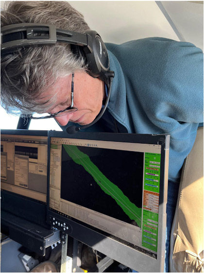
Goddard’s LiDAR, Hyperspectral, & Thermal Imager (G-LiHT) is an airborne instrument designed to map the composition of forested landscapes.
The G-LiHT instrument has a number of sensors that each serve a specific purpose. There are two LiDAR sensors that produce a series of LiDAR-derived forest structure metrics including a canopy height model, surface model, and digital terrain model. These models allow us to measure tree height and biomass volume.
Additionally, there are two cameras: one visible and one near-infrared (NIR). The visible and NIR bands acquired by the two cameras are paired to produce 4-band imagery. The 3-centimeter resolution photos taken by these cameras are aligned to build orthomosaics, which allow us to visually observe and identify changes in forest composition.
G-LiHT also has a hyperspectral sensor to acquire spectral information at a coarser resolution. These data can be used to identify vegetation composition and measure photosynthetic function as well as calculate vegetation indices at a fine spectral scale of 1 meter using radiometrically calibrated surface reflectance data.
The thermal sensor measures radiant surface temperature which allows us to create 3D temperature profiles derived from structure-for-motion. Thermal data provides us with information on the functional aspects of forest canopies. As photosynthetic function is related to evapotranspiration, we can observe that hotter canopies are more stressed relative to surrounding canopies.
The G-LiHT airborne mission supports multiple groups including the U.S. Forest Service (USFS), the USFS Geospatial Technology and Applications Center (GTAC), and the University of Alaska Anchorage.
The USFS is creating a forest inventory for the state of Alaska, and G-LiHT measurements collected over Forest Inventory and Analysis (FIA) plots are a cost-effective method of forest inventory. G-LiHT data will also help to improve regional estimates of aboveground forest biomass and terrestrial ecosystem carbon stocks. GTAC uses G-LiHT data measurements for algorithm development. USFS Geospatial Technology and Applications Center will use G-LiHT data acquired over FIA- and GTAC-measured ground plots and between these plots to map forest characteristics on federally managed lands, including forest type, biomass, vegetation structure, tree and shrub cover, and more. Data will also be used to guide future inventory efforts in coastal Alaska using methods developed for interior Alaska.
This field campaign also acquired repeat data over Fairbanks, Alaska, to measure changes in permafrost.
G-LiHT image data was reacquired over spruce beetle monitoring transects stretching from the Kenai Peninsula in the south to Denali National Park in the north. These transects were last measured on the ground and with G-LiHT in 2018, during the peak of a spruce beetle outbreak, and changes in vegetation structure and spectral reflectance will be used to evaluate the long-term mortality and growth of these forests.
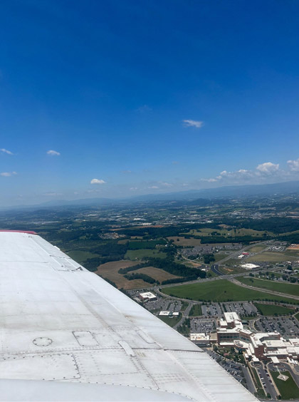
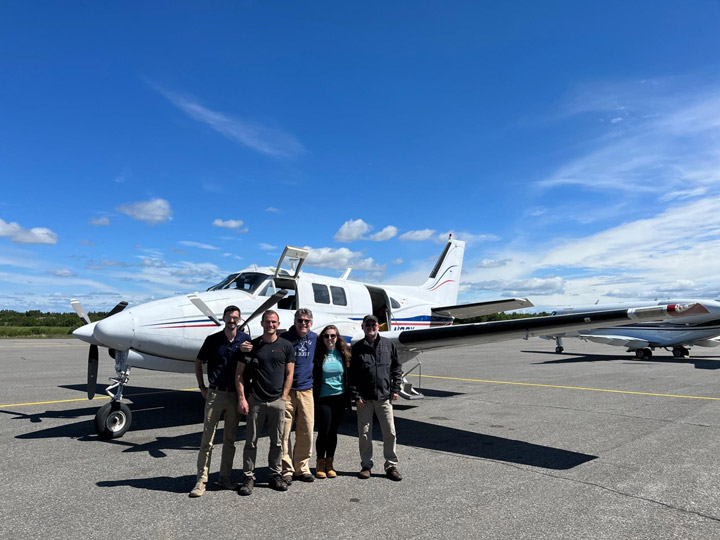
Our Alaskan field campaign started with an integrative test flight in June. Our team of three loaded up G-LiHT into a vehicle much too small and drove to Dynamic Aviation in Bridgewater, Virginia. We spent the first day installing the instrument into a 1960s King Air A90.
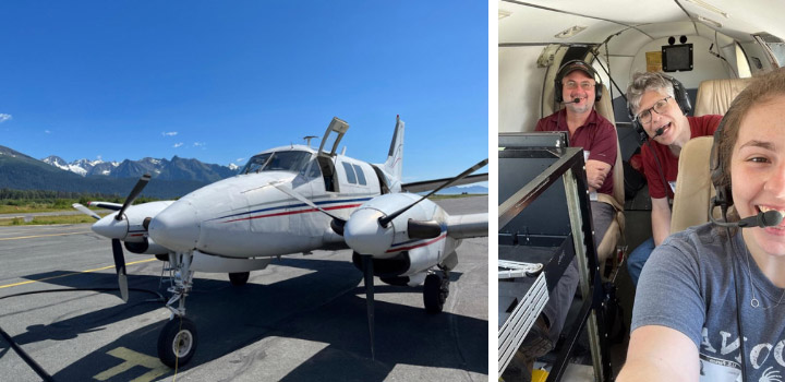
The second day was all about flying. We needed to make sure G-LiHT didn’t interfere with any of the aircraft’s systems. Additionally, the functional test flight over Harrisonburg, Virginia, allowed us to verify that G-LiHT was functioning properly. We flew in a grid pattern over the city which allowed us to geospatially align the data products from all of G-LiHT’s sensors.
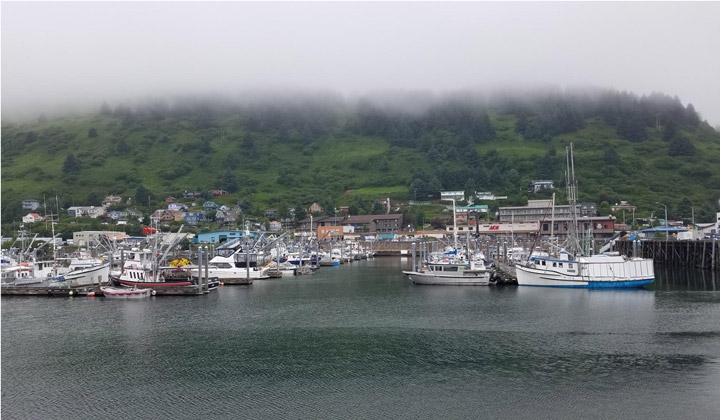
The integrative test flight was a success. We installed G-LiHT properly with no issues and obtained the information we needed. Once we received the thumbs up to proceed with our campaign, the pilots loaded up the plane with supplies and headed out to Kodiak, where we would meet them the following week.
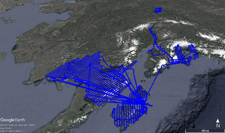
Our plan for the field campaign was to arrive in Kodiak, Alaska on July 6 and stay until the end of the month. We chose Kodiak as our hub because it was a convenient location to our flight lines. Unfortunately, despite the ideal location, poor weather prevented us from flying for the first three days of the campaign.
Once we were finally able to get in the air, we collected data over the forests near Iliamna.
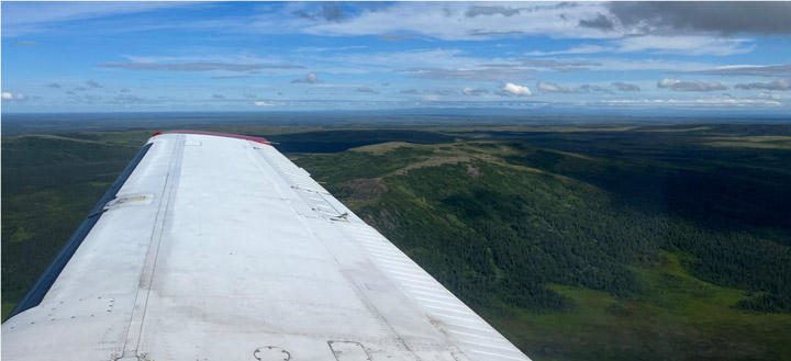
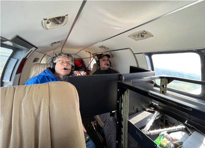
Most of our days consisted of our team meeting in the hotel for breakfast at 8 a.m., discussing weather and flight plans for the day, and then driving to the airport to prepare the plane and G-LiHT for flying. Depending on how many flight lines we were able to complete, we often stopped in King Salmon or Iliamna to refuel the plane and then went back out to fly more lines before returning to Kodiak.
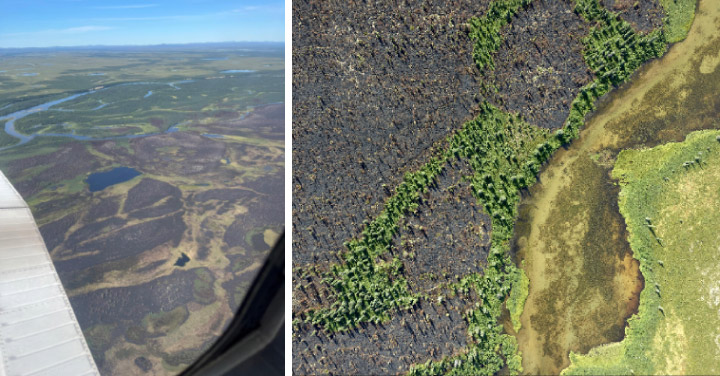
Our group was interested in measuring the effects of forest fires on vegetation in the Dillingham region. There were several burned areas to the west of the Nuyakuk River and east of Cook Inlet.
Toward the end of the campaign, we decided to transit to Fairbanks because the weather over the rest of our other flight lines didn’t look promising. If there were clouds below the plane at 1,100 feet, they would obstruct the instrument’s view and cast shadows on our data. We had to closely monitor the weather every morning. Additionally, we were unable to fly in rain or smoke as it would adversely affect the LiDAR sensors’ data returns.
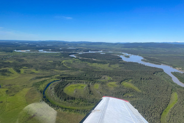
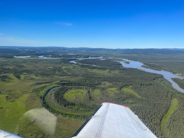
One geological feature we saw extensively in the southwest was the oxbow lake. Also called cut-off lakes, these lakes have formed when meandering rivers erode at points of inflection because of sediments flowing along them to the point where two parts of the river will join together, creating a new straight part of the river—essentially “cutting off” the curved lake piece. This created an oxbow lake. Once the lake has fully dried out, it becomes a meander scar. We noted the difference in vegetation growing back within the oxbow lakes and meander scars and how this differs from surrounding vegetation patterns.
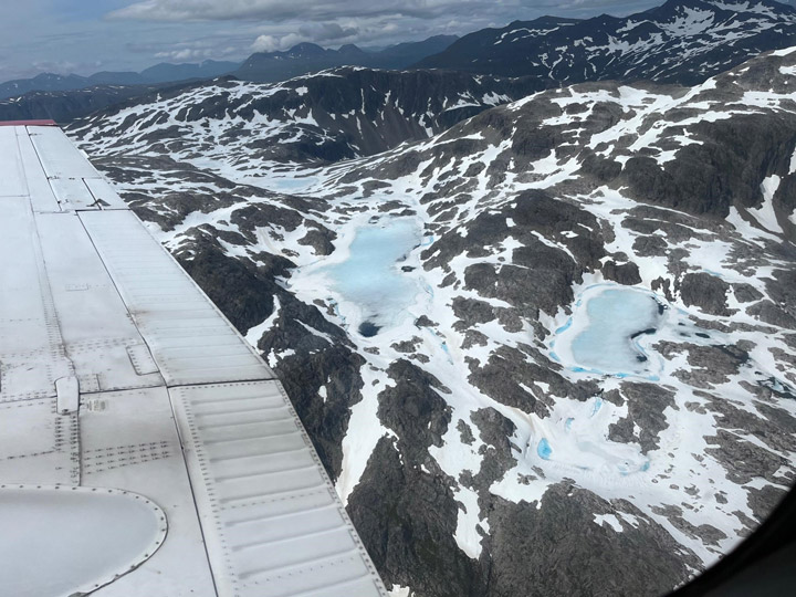
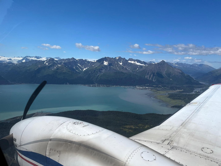
We had only planned to spend one night in Fairbanks, then transit back to Kodiak the following day. However, the weather had other plans for us. We ended up having to fly to Anchorage the following day because of extremely low cloud ceilings in Kodiak that made it too dangerous to land there. It worked out in the end, and the team was able to see more of beautiful Alaska and collect data over Anchorage and the Chugach region. It just goes to show how quickly things can change during a field campaign.
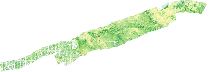
We collected data in the Campbell Creek region west of Anchorage. The data include visible and near-infrared photos which were composited into 4-band high-resolution orthomosaics and used to visually observe and identify changes in forest composition.
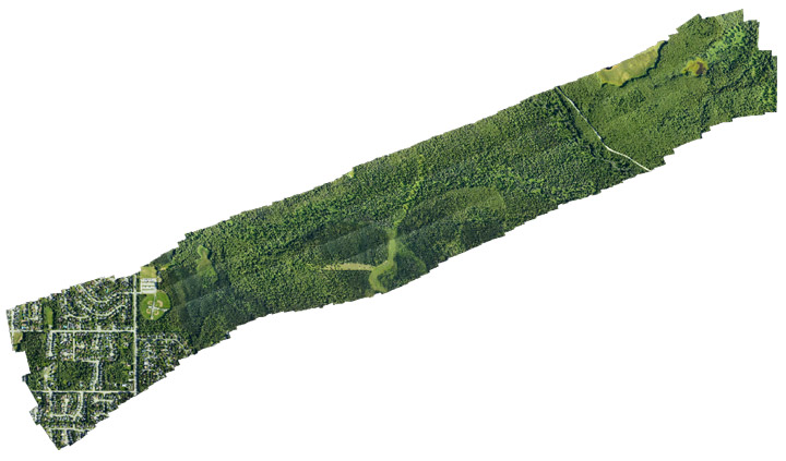
In addition to the high-resolution orthomosaics produced from the G-LiHT’s near-infrared and visible cameras, LiDAR data was processed to create various 1-meter resolution forest structure metrics including Digital Terrain Model (DTM), Digital Surface Model (DSM) and Canopy Height Model (CHM). These metrics are used to measure tree height and biomass volume. The CHM raster below was created by subtracting the DTM from the DSM.

After collecting data in Anchorage and the Chugach region of Alaska, the team flew back to Kodiak and finished data acquisition in the southwest.
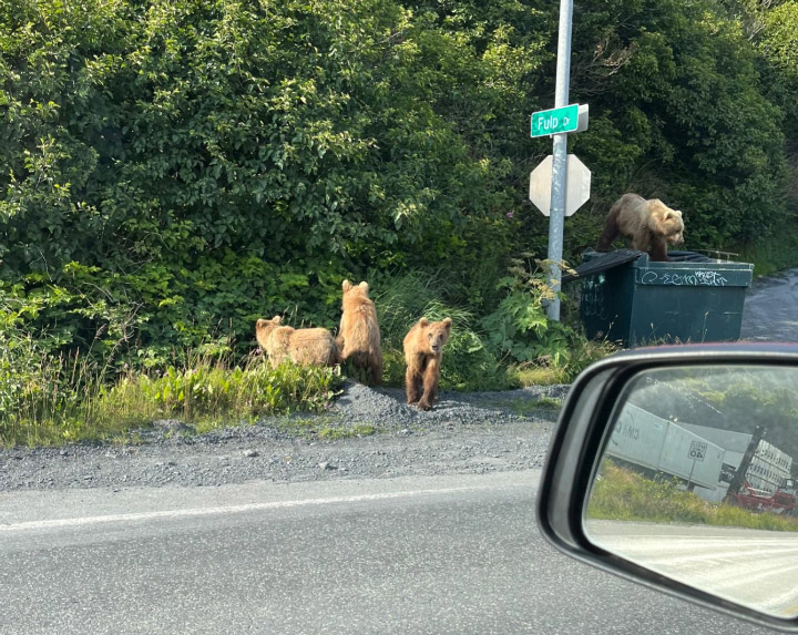
And of course it wouldn’t be Alaska without some wildlife. The day before leaving Kodiak, I got to see not just one bear—but a family of four! Cars were honking to scare the bears out of the road, but luckily I had enough time to snap a picture before the bears ran off into the woods. It was the perfect end to an exciting field campaign.
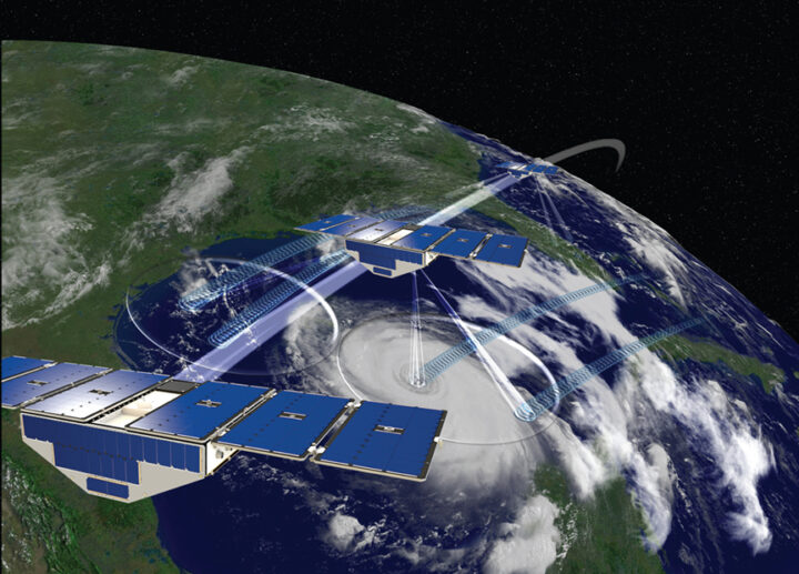
It’s been six years since the CYGNSS constellation was launched. Over that time, it has grown from a two-year mission measuring winds in major ocean storms into a mission with a broad and expanding variety of goals and objectives. They range from how ocean surface heat flux affects mesoscale convection and precipitation to how wetlands hidden under dense vegetation generate methane in the atmosphere, from how the suppression of ocean surface roughness helps track pollutant abundance in the Great Pacific Garbage Patch to how moist soil under heavy vegetation helps pinpoint locust breeding grounds in East Africa. Along with these scientific achievements, CYGNSS engineering has also demonstrated what is possible with a constellation of small, low cost satellites.
As our seventh year in orbit begins, there is both good news about the future and (possibly) bad news about the present. First the bad news. One of the eight satellites, FM06, was last contacted on 26 November 2022. Many attempts have been made since then, but without a response. There are still some last recovery commands and procedures to try, but it is possible that we have lost FM06. The other seven FMs are all healthy, functioning nominally and producing science data as usual. It is worth remembering that the spacecraft were designed for 2 years of operation on orbit and every day since then has been a welcomed gift. I am extremely grateful to the engineers and technicians at Southwest Research Institute and the University of Michigan Space Physics Research Lab who did such a great job designing and building the CYGNSS spacecraft as reliably as they did. Let’s hope the current constellation continues to operate well into the future.
And finally, the good news is the continued progress on multiple fronts with new missions that build on the CYGNSS legacy. Spire Global continues to launch new cubesats with GNSS-R capabilities of increasing complexity and sophistication. The Taiwanese space agency NSPO will be launching its TRITON GNSS-R satellite next year, and the European Space Agency will launch HydroGNSS the year after. And a new start up company, Muon Space, has licensed a next generation version of the CYGNSS instrument from U-Michigan and will launch the first of its constellation of smallsats next year.
The CYGNSS team will continue to operate its constellation, improve the quality of its science data products, and develop new products and applications for them, with the knowledge that what we develop now will continue to have a bright future with the missions yet to come. Happy Birthday, CYGNSS!
