NASA’s DC-8 is usually the aircraft flown from South America to Antarctica for the IceBridge mission’s annual research flights over the continent. But this year, the DC-8 was booked for a different mission, so NASA’s P-3 filled in. Since late October, the P-3 crew and instrument operators have been making flights out of Ushuaia, Argentina, to map Antarctica’s ice.
The scenery outside is stunning and the amount of data collected enormous. But as often as people ask about Antarctica and the mission’s science goals, people also want to know about P-3. As the following images show, this is not your typical aircraft.
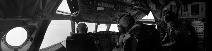
Here’s a peek inside the P-3 flying research laboratory, from front to back.
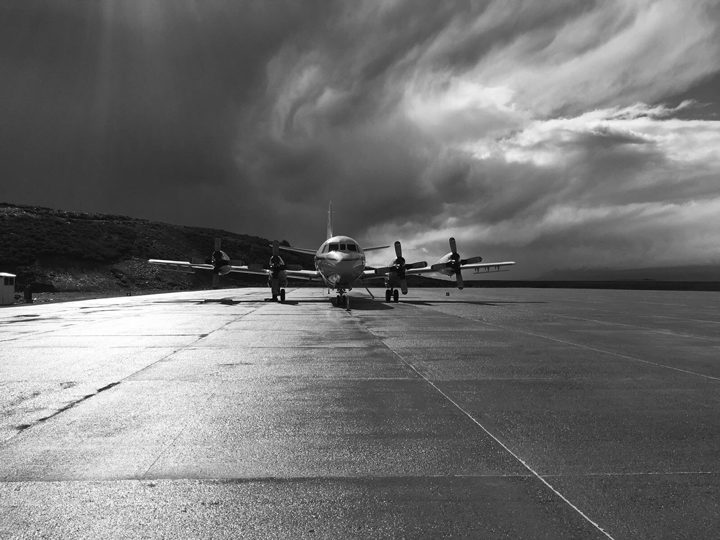
The NASA P-3 sits on the ramp at the airport in Ushuaia, Argentina. Photo by Aaron Wells/Indiana University.
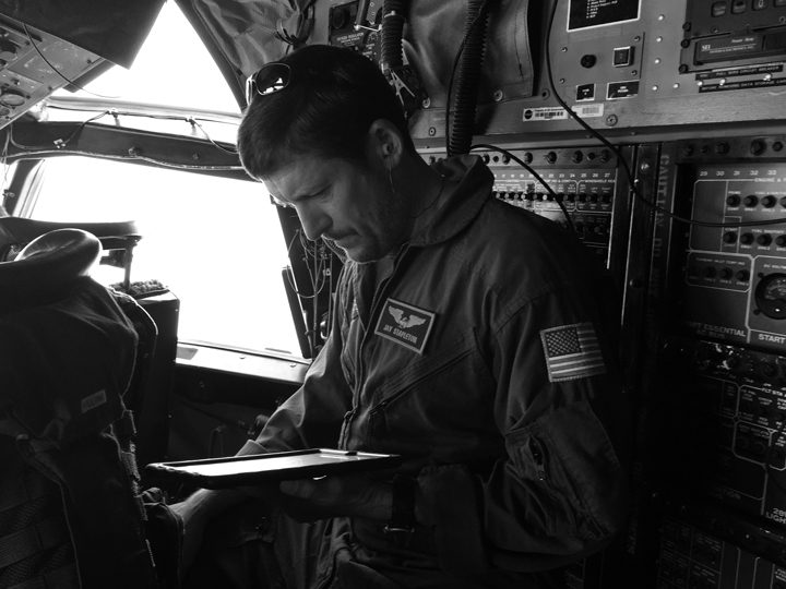
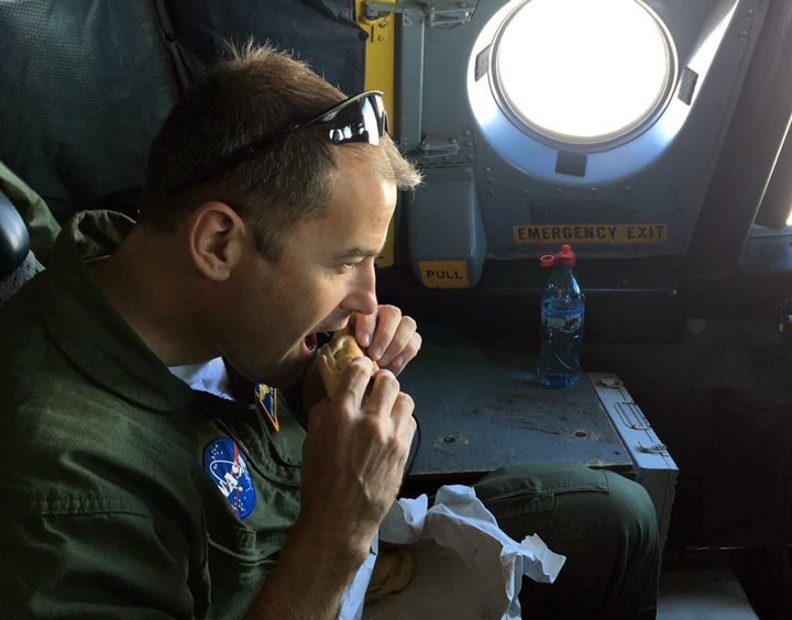
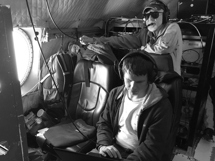
NASA pilot Jay Stapleton waits to fly. Pilots work in shifts during the nine-plus hour flights.
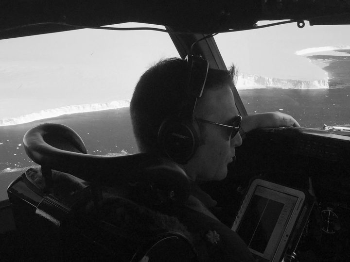
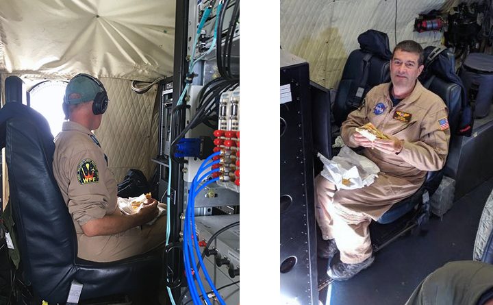
NOAA pilot Patrick Didier flies the P-3 during the November 12, 2017, flight over the Larsen C ice shelf.
John Sonntag, NASA IceBridge mission scientist, monitors data collected during a research flight on November 12, 2017.
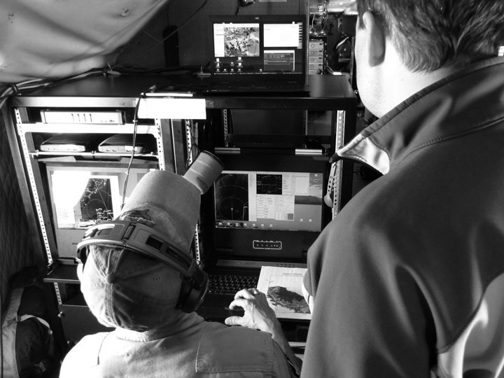
IceBridge project scientist Nathan Kurtz (front), and Dennis Gearhart of the Digital Mapping System (DMS) team (back) monitor imagery acquired during the research flight on November 14, 2017.
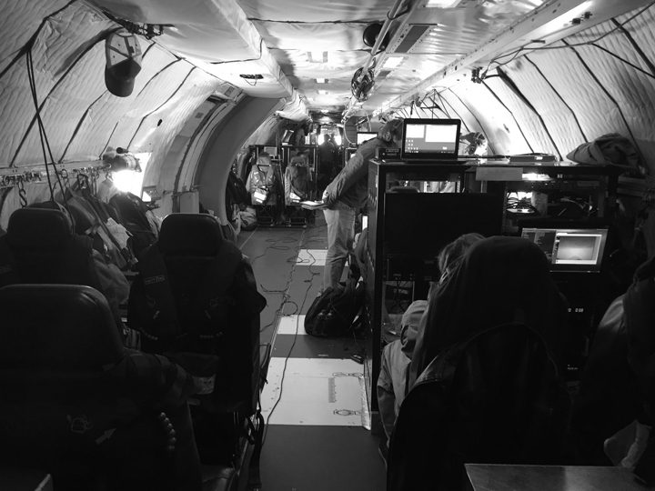
The view from the back of the P-3 shows how the aircraft has been modified to support racks of computers and science equipment.
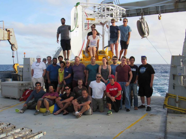
Kyla Drushka, Chief Scientist SPURS-2 2017.
This will be my last blog from R/V Revelle and SPURS-2. Overall, we had an excellent and successful expedition, ably led by Kyla Drushka of University of Washington. This is a good time to give you a thumbnail sketch of accomplishments and tie up loose ends.
Here is a quick summary of key data collection systems:
The underway CTD team completed 501 casts. At rates of 2 per hour while “speeding” at 10 mph and 1 per hour at 4 mph, that amounts to many hours of standing on back deck, rain or shine, night or day. The UCTD team gets kudos from the entire SPURS-2 team for a job well done.
We deployed the Surface Salinity Profiler 16 times. It worked very well once some initial bugs were worked out. The laser and imager were deployed for all the SSP runs.
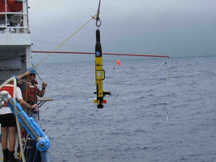
Almost all SPURS-2 instruments were recovered. All three moorings came back whole and in working order. Lots of valuable time series data to examine. Of the three Wave Gliders deployed in August 2016, two worked the entire 15 months until we recovered them this voyage. One WaveGlider lost its lower half after a couple months. The Lady Amber recovered the upper portion. SeaGliders worked very well and were recovered.
The SEA-POL radar was an great addition to the voyage and worked seamlessly. Kudos to the team from CSU, led by Steven Rutledge, who all performed so well on their first sea experience with SEA-POL.
Meteorological data and air-sea exchange information were collected the entire voyage. Radiosondes were deployed 4 times per day to contribute to the global network and provide valuable background for the SEA-POL.
The Salinity Snake and thermosaliniograph systems also performed very well. On this voyage the snake system also supported work by David Ho and Sophie Clayton on CO2 and biology respectively. Kudos to Julian Schanze for advancing the Salinity Snake technology (better on every deployment since 2012).
Were there losses or failures? Some SSP parts were lost when when an electronics box leaked; the salinity rake (tested on a Wave Glider) again had leakage issues but did collect a couple of days of interesting data; a Wave Glider failed early in SPURS-2; our planned drifter experiment was severely reduced in scope due to failure of the GlobalStar positioning system coverage for 25 of 35 drifters. The drifter “outage” may have been due to the San Martin, Mexico gateway Earth station being taken out in a recent earthquake, but that is not confirmed.
There are interesting science stories that will emerge as analysis gets going:
Sampling in rain and low wind yielded a large number of observations of “puddles” (steep salinity gradients in the upper 5 m due to rain). Many SPURS-2 scientists will contribute to the analysis including Kyla Drushka, Julian Schanze, and Ben Hodges. Bill Asher will tie surface turbulence estimates to the puddle observations.
The observation of rain rates and rain drop characteristics with the SEA-POL radar will greatly enhance the oceanographic analysis of the near surface ocean. Elizabeth Thompson will work to link the atmospheric measurements to the oceanography. Steve Rutledge and his team will likely publish new findings about convection characteristics in the ITCZ.
The large-scale characteristics of the east Pacific “fresh pool” are documented in numerous U-CTD transects. Janet Sprintall and others will illuminate the relationship of the fresh pool to the ebb and flow of the North Equatorial Current and the North Equatorial Countercurrent.
The 14-month time series of moored measurements will yield valuable information on seasonality and mixing in the fresh pool. Tom Farrar and Billy Kessler will be working with many other investigators because the time series over an entire year puts all the expedition specific collections in context.
The impact of rain on the ocean surface partial pressure of carbon dioxide was documented in observations for the first time by David Ho.
The biogeography of plankton in the Eastern tropical North Pacific was greatly enhanced by extensive collections and photographs by Sophie Clayton.
We all must thank Kyla Drushka, our Chief Scientist, for keep all the projects happy and coordinated. It was her first time in this role and she did an awesome job.
And here are some loose ends:
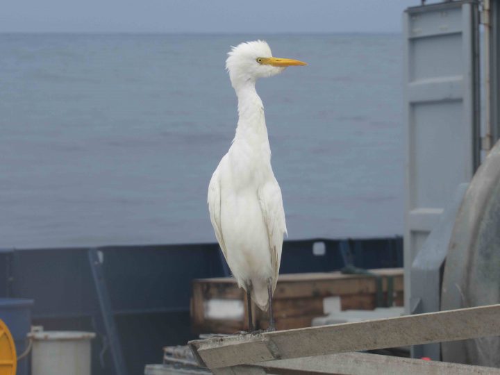
A cattle egret standing tall.
+Egrets – They are Cattle Egrets stupid, not Great Egrets. We had two aboard for weeks, then a third one appeared, but he or she did not stick around. Thanks to all the interested birders out there who rectified my identification miscue. Trina Litchendorf played caretaker to the birds. They stuck to her like glue whenever she was on deck. She had a fabulous egret costume for Halloween. Her care for the birds was touching. Thanks Trina!
+Peruvian Booby – This bird hung around for quite a while, but eventually disappeared. Sorry to say, he was looking worse for wear. Let’s just say, I fear, that he took the ultimate Booby Prize.
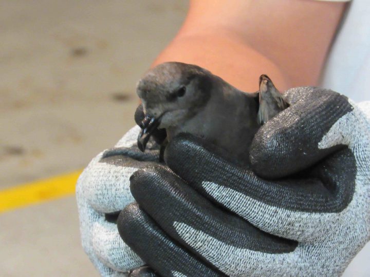
+Black Storm Petrels – We have caught and released a significant number of these small black birds. They crash into the ship at night and we find them stunned on the deck. All have been re-launched into their ocean realm.
+Flying Fish – Finally got a picture of a school in flight! It is fun to watch them, but exceedingly difficult to photograph them. I finally got lucky and share the photo with you.
Also a Haiku:
Flying fish skitter
Scaly bullets piercing air
Aloft a silent team
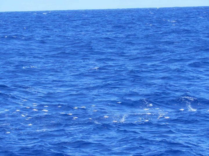
An armada of flying fish.
So, dear readers, I think my prose is done. I know so because I am leaking Haiku. The voyage has worn us out. We are still enthusiastic, but it is muted for all by the tyranny of producing 24/7 week upon week. Channel fever (See prior blog: Channel Fever as an Expeditionary Malady) is sweeping the ship. Homeward bound we fly. The reality of what was accomplished in SPURS-2 is yet to sink in. Scientific papers are only a dream right now. Authors must sleep on the results a bit. Then return with fresh enthusiasm to analysis and writing!
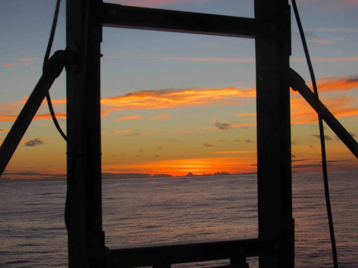
The Sun sets on the SPURS-2 expedition.
Fair winds and following seas to all!
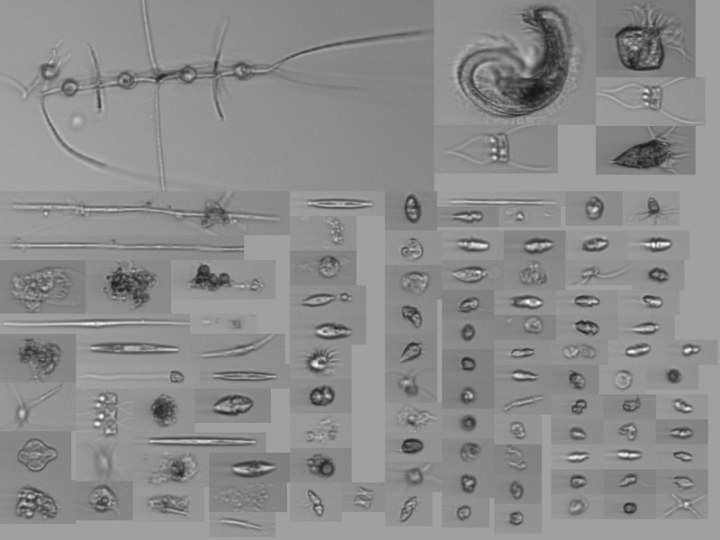
A mosaic of pacific_plankton from a single sample.
Who lives down below us? This is a question that mariners have wondered for ages. We no longer think of the darker answers to this question – of the sea monsters, the Kraken, the great whales. For most aboard, the thinking is that of the fisherman – of the tuna, mahimahi, and sharks. For SPURS-2, Sophie Clayton is answering this question in terms of the microscopic life below us – of diverse phytoplankton (plant life) and zooplankton (animal life).
Sophie is an oceanographer interested in understanding how ocean currents at all scales shape the distribution and biodiversity of phytoplankton. She uses a combination of numerical models, large scale data analysis and targeted observations made at sea. Her Ph.D. in Physical Oceanography from the MIT/WHOI Joint Program. Now she is a postdoctoral fellow at the University of Washington, working extensively with observations of phytoplankton distributions made using an imaging flow cytobot (IFCB) that analyzes discrete samples with video and a hyper-spectral optical sensor for recording the continuous optical properties of the water.
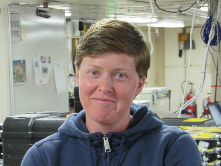
Sophie Clayton at work in Revelle laboratory.
An IFCB is an instrument that is used primarily to count cells, but it also can detect and record information on different properties of the cells that it counts. A water sample is channeled into a thin stream that is passed in front of a laser, and the scatter and fluorescence from each cell that passes along the stream in detected and recorded. In the IFCB, the camera is triggered to take a picture only when fluorescence over a threshold value is detected. This means that the instrument only takes pictures of cells that contain chlorophyll. The images are then stored for analysis back on shore. As well as the images that are collected, we use the optical properties of the cells (fluorescence and scatter) in the analysis.
Sophie’s work is enabled by surface water collected (from the salinity snake) while we are underway or from bottle samples taken during CTD casts. A sample mosaic image from the cytometer is shown here – representing material sampled from one bottle of seawater collected by during a CTD cast. Similar mosaics are made from surface water ever 20 minutes. Overall there will be close to 2000 mosaics of cellular life to examine. Samples are also held for later DNA analysis.
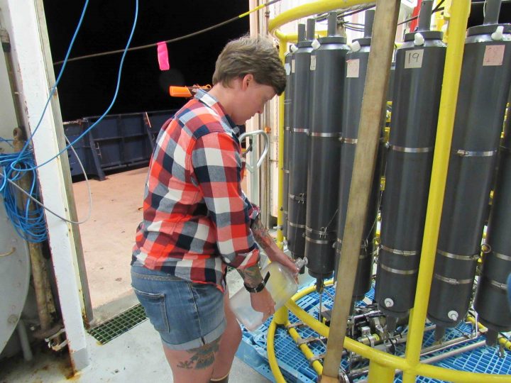
Sophie collecting a 4 liter bottle of seawater for filtering.
Out here, for the most part, the plankton are actually most abundant below the surface at 40-70 meters depth. Deeper down, below the surface layer mixed by the wind, life has better access to the chemical nutrients of the deep sea – while still having enough light for photosynthesis. Plant life thrives in a layer that best balances the light and nutrient requirements. Of course the grazing microscopic animals follow this layer closely. So, Sophie is keen to collect water from this layer during our CTD casts. She can tell where to sample by optical properties also measured on CTD casts.
Understanding plankton abundance and diversity is a core requirement for ocean climate science. Phytoplankton are responsible for about half of all photosynthetic production on the planet (land plants are also responsible for about half). It makes them a key part of the carbon cycle on the planet. Over long periods, phytoplankton can remove carbon from the upper ocean and return it to sediment for long-term sequestration. Over hundreds of thousands of years, phytoplankton act to reverse the greenhouse effect caused by pulses of carbon dioxide injected into the atmosphere by volcanoes or humans.
There are always meticulous notes to keep about samples.
In a prior blog (See Whither Life in the Sea) I wondered about the fate of life in the sea. What would become of the abundant life in the sea with the continued impacts of ocean acidification, industrial fishing, and plastics pollution? Science struggles to make any predictions. Oceanographers particularly, because of our close affinity and observation of the sea, hope that the assaults of society on the sea do not damage its inherent ability to stabilize and heal the rapid changes overtaking the planet. Our baseline understanding of the complex marine ecosystem is still quite primitive. The kind of “survey” work that Sophie is undertaking are absolutely necessary to further our understanding of the biogeography of the ocean and how it is changing. Lets hope she has a successful career!
Ecomapper with the salinity snakes.
As the Program Manager at NASA Headquarters responsible for our satellite mission (Aquarius) dedicated to measuring the surface salinity of the ocean, I set in motion some work to better understand and measure surface salinity directly, at sea. Even as Aquarius ended in 2015, its role has been filled by another mission (SMAP), so the intense study of surface salinity and what it tells us about the water cycle on Earth continues. These missions, their NASA program manager, and the community of science have spun off a new “cottage industry” (as space missions often do).
The central question motivating the industry is, “who can provide NASA with actual sea-truth on the sea surface salinity?” Buried in the answers to that question is the growth of new technology and some very challenging field work!
SPURS-2 is the apogee of this new industry. Aboard Revelle, we have all manner of ways to sample the upper-most layer of the ocean, away from the disturbances of the ship. The objective is to see “the things we see from space” but could not observe before with older oceanographic technology.
Julian Schanze.
Before proceeding, you need a super-short physical oceanography lesson. The upper ocean is mixed by the wind. This “mixed layer” may be quite deep – hundreds of meters – for example, under winter storms with weak insolation by the sun. The mixed layer may be quite shallow or non-existent when there in little or no wind, and when there is heating or fresh water input at the surface. Wind over much of the ocean is sufficient to keep the upper 5-10m mixed.
Thus, for much of the ocean the “sea truth” for surface salinity is the same as having a salinity in the mixed layer. Argo floats, of which there is a standing flotilla of around 4000 in the ocean, measure salinity in the upper ocean between 2000m depth and about 5 m depth. They shut-off in the last five meters before they surface, to transmit their data, in order to protect their sensitive salinity-measuring cell against the bio-films on the ocean surface. So, they provide a great estimate of surface salinity everywhere in the ocean where the mixed layer is greater than about 5 meters. That is a very large portion of the ocean! Argo is the workhorse for calibrating salinity missions against “sea-truth.” But it leaves us with some unanswered questions.
What remains is what has spawned our small cottage industry. We can see from space that there are significant areas of the tropics where surface salinity is much less than indicated by Argo maps of “surface salinity” (really 5 m salinity). What is really going on there and why isn’t the Argo system working for us? What was discovered is that in these particularly rainy parts of the planet (mostly the Intertropical Convergence Zone), where their are low winds, the salinity of the upper ocean is lowered by rainfall quite dramatically and that fresh water can ride upon the salty water below quite well until wind picks up to mix it down. From space one can see a variable and dynamic “East Pacific Fresh Pool” that rides atop the ocean regularly monitored by Argo. The same phenomenon happens with large river plumes that reach the open ocean (such as the Amazon, Congo, or Mississippi) where satellite salinity is measured.
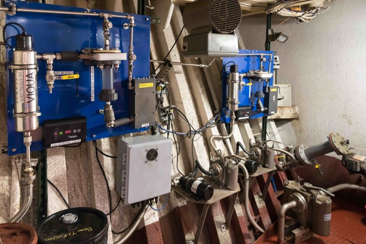
The thermosalinography system in the bow of Revelle. (Photo by J Schanze).
The “cottage industry” has manufactured ways to measure and monitor the phenomenon of this “fresh pool” with shipboard and autonomous platform technology. For examining fresh “puddles” and the larger fresh “pool”, the Revelle has “extra” salinity sensors in its bow to measure at 2m, 3m, and 5m depths. Julian Schanze has added on an outboard boom “the salinity snake” to catch and measure water from the surface. The UW APL team led by Kyla Drushka has the Surface Salinity Profiler to measure salinity at many levels from the surface to 1 m depth. A WaveGlider has been outfitted with a salinity “rake” to measure salinity at 10 levels in the upper 1 m. Ecomapper can be set on a mission to profile the upper few meters of the ocean for hours at a time. Finally, this issue has also spawned new Argo floats that measure salinity in the upper 5 m without compromising there “deeper” mission. SPURS-2 is the expedition to the East Pacific Fresh Pool that assembles all these good works of the “measure salinity in the upper 5 m of the ocean for NASA” scientific community.
Julian has prepared a plot showing salinity in the upper 5 m during one of the rain events sampled by Revelle. It shows one a plot of salinity (in color) versus depth in top 5 m and distance along track. The event or “puddle” has low salinity in just the upper 2 m or so, spread over about 5 km of distance. These are exactly the kind of features that would be missed by a standard Argo float but show up in satellite data.
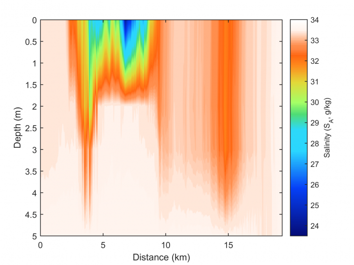
We return to shore with a data set rich in information about the workings of rain, surface salinity, stratification of salinity in the upper ocean, and upper-ocean mixing. From its analysis we will better understand the east Pacific as seen from space and know how to validate the salinity products from Aquarius and SMAP for these special areas. Ultimately these results help us understand the ocean’s role in the global water cycle. Not bad for a cottage industry spun off from the space program.

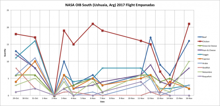
In the nine-plus hours it takes to fly from Argentina to Antarctica, collect data over the continent and fly back again, people on board are bound to get hungry. There is a microwave on board, as well as some snacks and hot drinks. But there are no flight attendants, and there are no meal carts. NASA’s P-3 is equipped primarily for science.
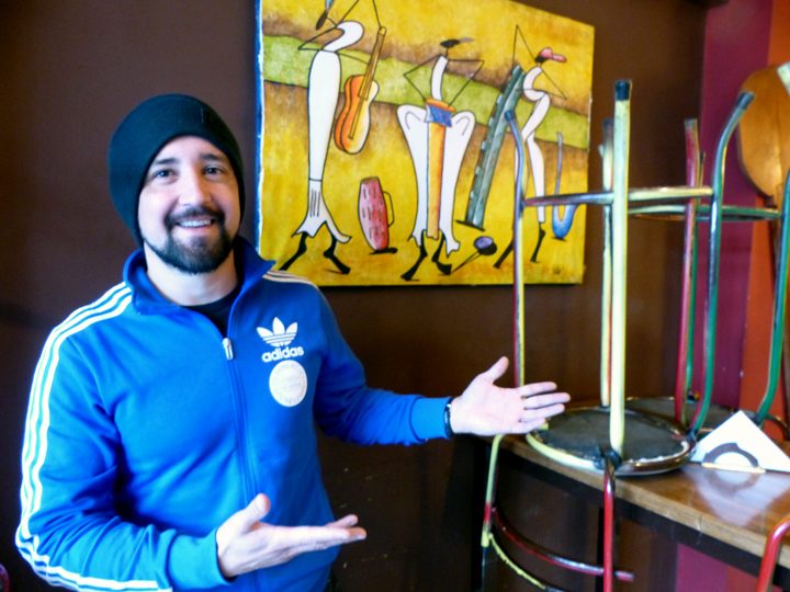
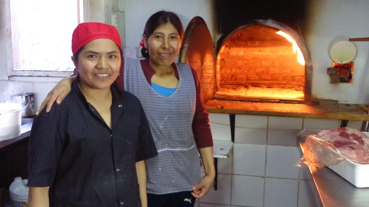
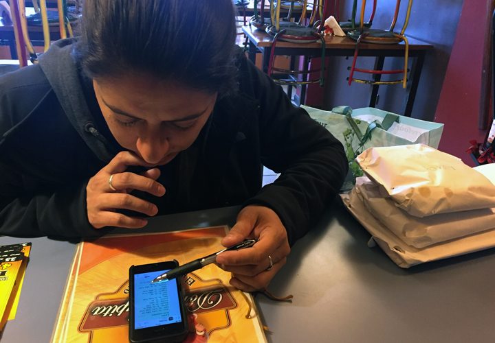
But that doesn’t mean instrument operators and crew go hungry. In addition to working with the airport and local government to ensure paperwork is in order, Operation IceBridge deputy project manager Eugenia De Marco also takes on the task of ordering and procuring daily orders of … what else … empanadas. And she approaches the task like only an engineer would.
Every evening, De Marco opens an Excel spreadsheet and records the orders of approximately 15 people. The orders are tallied and delivered via text message to Nicolas Furlanetto, owner of Ushuaia restaurant Doña Lupita. The next morning, Furlanetto and his staff arrive at the restaurant by 6:30 a.m.—hours earlier than on a typical day. Anywhere from 23 to 85 fresh empanadas are lifted from the wood-burning stove, neatly wrapped in paper, and labeled with our names.
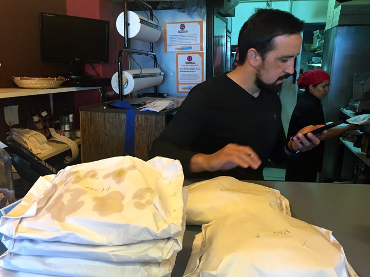
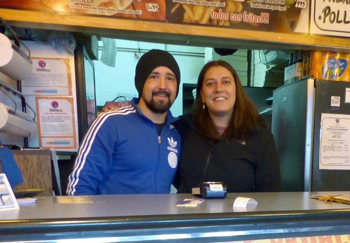
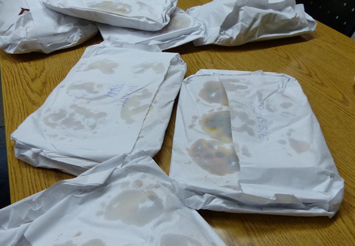
If none of the 11 varieties of empanadas speak to you, pizza and sandwiches are options too. But most of us stick with the empanadas, filled with everything from beef to Roquefort cheese. According to Furlanetto, the “matambre” and “carne a cuchillo” are the varieties most often ordered by locals. Our group bucks the trend. De Marco prepared a chart based on our empanada order history, and the data show chicken is the clear winner.