By Ryan Walker
Credit: NASA/Christine Dow
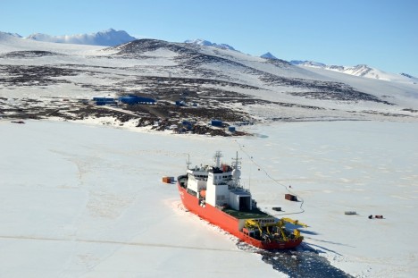
Before it was time to recheck our GPS stations and download data from them, the icebreaker Araon arrived at Jang Bogo, bringing new scientists, a new helicopter crew, fresh food, and other supplies. Because of heavy sea ice cover on the bay, the arrival was in slow motion, taking most of a day from the time the ship was visible from the station until it stopped a few hundred yards offshore due to unbreakable eight-foot-thick ice. Thick ice often requires an icebreaker to back up a considerable way, then charge forward into the ice, breaking through either by pure impact or by sliding the bow up onto the ice, causing it to collapse under the ship’s weight. One passenger told Christine and me that it was “like being in a car crash — all day.” We’re quite happy that there will already be a clear path out of the bay when we take the Araon back to Christchurch. Before leaving again for a roughly week-long science cruise, the ship also dropped off quite a lot of equipment for the various science teams, including most of the instruments to be installed by our hosts, the Extreme Geophysics Group. This meant that the time between Araon’s departure and return would be very busy, with limited time to install instruments before most of the scientists leave on the ship. On top of this, we had several days of bad weather that prevented any helicopter flights. In order to finish our work on the GPS stations, we had to squeeze into a busy flight schedule, which meant that Christine and I would go on separate flights.
Credit: NASA/Christine Dow
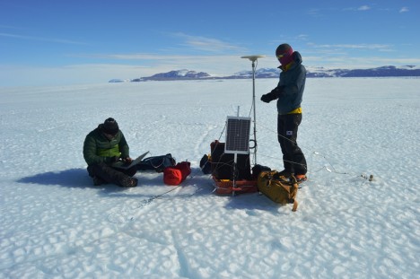
I was on the first flight on December 10, which began with Dr. Choon-ki Lee installing a new GPS station on a large piece of ice at the front of Nansen Ice Shelf that looks ready to calve off into a tabular iceberg. There’s a huge crack, miles long and sometimes over a hundred yards wide, which runs more or less parallel to the front of the ice shelf. Over the winter, the sea surface freezes and traps small icebergs in the crack, producing a fascinatingly broken icescape. Comparing ice velocities between this new GPS and our stations should let us monitor the calving process and learn more about how it works. When we moved on to check the first of our GPS stations, I found that it wasn’t operating at all. After checking the wiring, I worked out that the problem was either in the wire to the receiver, the regulator (the electrical component that connects the solar panel, battery, and receiver), or the GPS receiver itself (potentially big trouble) — but had no idea which one. I pulled out those three components to check back at Jang Bogo, and we secured the rest of the station and moved on. Fortunately, after an unpromising start, the two other GPS stations we visited were working perfectly. While downloading the data, which involved about fifteen minutes of connecting my laptop and then sitting on the ice typing obscure commands, I was amused by how much this aspect of field work resembled the computer modeling work I usually do, though with vastly better scenery. We then returned to Jang Bogo with two stations in good shape, two yet to be checked, and one hopefully to be repaired.
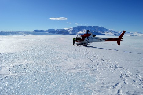
Christine says: It was getting worryingly close to the time when we would be leaving the Antarctic and we still had some data to collect and the GPS to fix. I found that the GPS problem had been due to a faulty solar regulator and replaced it with a spare back at base. Luckily I managed to piggy back on a flight out to the Nansen Ice Shelf with the Extreme Geophysics Group while they were putting out seismic stations. Replacing the GPS was quick, with the satellite lights blinking encouragingly; now we just have to hope the system will continue working for the next couple of months. At the next station, I downloaded the data while wind blew some loose snow all over me and the computer. I probably looked a little like a snowman by the end of that. The final job was to replace the tethers on the last GPS (see our previous blog post). It was not without sadness that I waved goodbye to the plucky little machines, which would sit out on the ice on their own until the end of February. At that stage one of our Korean colleagues who is overwintering at Jang Bogo will collect them for us and send them back on the ship.
Speaking of the ship, we’re off. It is due to arrive tomorrow and we will set sail for our 7-10 day ‘cruise’ back to Christchurch in New Zealand. Its hard to believe we’ve been here 5 weeks already and it feels a bit strange to be packing up and leaving. We’re hoping for some wildlife spottings on the boat and more importantly not to be completely debilitated by sea sickness. Internet is not readily available on the Araon so we will report back when we reach dry land. Wish us luck!
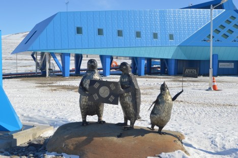
Goodbye, Jang Bogo! (Credit:NASA/Christine Dow)
By Christine Dow
Credit: NASA/Christine Dow
The big day had arrived. We were due to fly to our tiltmeters to collect the data that they had been gathering for two weeks. once this was the first time we had ever set these instruments up in the field, all fingers were crossed that we had been precise enough in initially leveling the meters so the data were in range and also that the solar panels hadn’t ended up covered in snow.
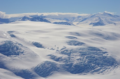
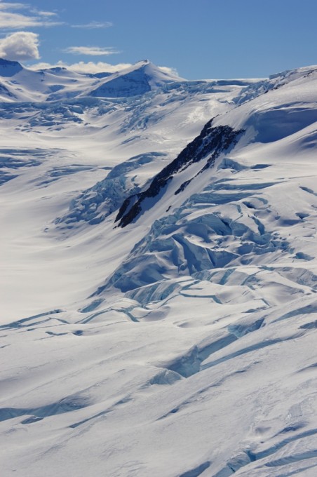
We had a spectacular flight, cutting over the end of Priestley Glacier and skirting helicopter-sized crevasses on the mountain behind our field site. Despite a bit of wind on the Nansen ice shelf, it was as calm on the Comein Glacier as it has always been for our visits. It’s such a peaceful, sheltered spot that I feel a holiday cottage wouldn’t be amiss. Perhaps too long of a commute for an average Friday afternoon, however.
Credit: NASA/Christine Dow
One of the tiltmeters (which are in black boxes) had become exposed and, because black materials absorb heat whereas white materials reflect it, had caused a bit of local melt which had trickled down the side of the box and refrozen. The upshot of this was that the entire box, battery, and straps were encased in some pretty solid ice. Fun! Commence some delicate hacking with ice axes so that we didn’t snap the wires coming out of the box. Finally having reached the interior, we nervously extracted the SD card and Ryan pulled the data off onto the computer. Success! Some excellent (and exciting) looking data showing tidal cycles. Tiltmeter two was easier because it hadn’t caused local melt of the snow so we could quickly retrieve the data. Again, some very interesting outputs. We want to thank John Leeman, an engineer from Penn State, for building us some happily working tiltmeters. Of course having disturbed the tiltmeters I had to reset them back to full level, which required sitting for 10 minutes enjoying the view while very delicately adjusting the little leveling legs.
We had just enough time to collect data from one of the GPS closest to the tiltmeters. All looked well apart from our tethers, which had come loose because of melt on the surface. We had one bamboo tether and one metal peg. The metal had heated up and melted a groove in the ice as it was pulled along, whereas the bamboo had stayed where it was supposed to. We tightened the wire as much as possible but we would have to return to this site with some more bamboo later.
Credit: NASA/Christine Dow
Dinner back at base was a happy affair, having achieved success for at least three of seven of our instruments. The chefs had even made some pizza for us, which was a nice treat. The only unfortunate aspect of the day was that I had forgotten that in areas with 24 hour sunshine and highly reflective snow surfaces it is essential to put sunscreen up your nose as well as on it. Burnt nostrils are not fun, but they’re worth it for some nice data.
Today’s post will be a ‘guest’ post from Luke Madaus, expert weather forecaster, numerical modeler and graduate student from the University of Washington.

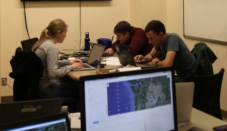
The OLYMPEX forecast team. From left: Sarah Bang, Leah Campbell, Nick Weber, Jen DeHart, Luke Madaus and Joe Zagrodnik. Not pictured: Peter Veals and Trey Alvey.
A Day in the life of an OLYMPEX forecaster by Luke Madaus.
When people think of field campaigns, they usually think of windblown scientists, struggling against the elements to get those critical observations of the fantastic weather surrounding them. Be it flying in planes, scanning with a radar or fixing a ground station, all these intrepid scientists would be nowhere unless they had some idea of what was coming at them, weatherwise.
That’s where we come in.
We are the forecasting team, the unsung (or, at least, the background chorus of) heroes that don’t actually get out into the field, who rarely leave the climate controlled operations center, but provide the critical guidance that’s needed to make sure the day goes smoothly. Here’s what a day in our life is like.
The time our day begins as a forecaster depends on what’s going on that day in the field operations. If there are aircraft involved, we may have to be ready to go in the middle of the night, as a 3 hour preflight forecast is needed to evaluate last minute changes and reaffirm the safety of the flight. But let’s say for now that today is a day where the planes are not taking off early in the morning. In that case, the lead (and helper) forecasters arrive around 7 AM to get a head start looking at the latest weather model runs. We work together to discuss the latest model forecasts and what they’re showing. Here at the OLYMPEX operations center we keep a running timeline of the next five days or so, updating it as new forecast models come in and our perception of the forecast changes.
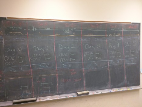
The timeline is updated every day and shows the timing of storm systems by various forecast models and timing of radar and aircraft operations.
The main goal for the first few hours of the morning is to become familiar with the current observations, latest model runs, and then prepare that information for the morning weather briefing. Our task for this briefing is to develop a narrative timeline for the next several days of what to expect over our study area. For instance…when is the next cold front due to arrive? How long will the frontal precipitation linger? Will there be any postfrontal showers? Interwoven with that are evaluations of potential hazards for the field campaign operations. For example, recently we’ve had lake flooding nearly drown the Doppler On Wheels radar and high winds have kept planes grounded when we wanted them to fly. Any possibility of hazards to operations needs to be voiced.
Forecasters getting ready for the morning briefing, Jen Dehart (left), Luke Madaus and Nick Weber (right).
We’re also challenged to present the uncertainty in the forecast. We look at multiple models, both deterministic and from ensembles, to assess confidence in the narrative timeline we are developing. Sometimes it’s easy, sometimes it’s a challenge. For instance, here are two model forecasts for sea-level pressure and 10m wind speeds along the western Washington coast. On the left is a 36 hour forecast for one afternoon, on the right is the forecast from the next model run. Surprise! A low pressure center with strong winds is now indicated! It’s our job as forecasters to assess the likelihood of these various scenarios and report on what we think will happen (and our confidence levels) to the mission scientists.
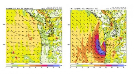
Two model forecasts valid at the same time. The one on the left shows light to moderate winds. The one on the right shows a developing low and strong coastal winds. Which one will be right?
That responsibility continues through the morning weather briefing, when the mission scientists review our forecast narrative and ask us questions. How certain is the forecast? What is the expected structure of the precipitation? Will it rain or snow in the mountains? Will the convection be deep or shallow? This is what we’ve been preparing for as a forecaster all morning so we are able to say, “Aha! I have the answer for you!” and impress the operations and flight directors.
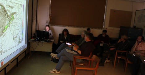
Jen DeHart gives the morning briefing while operations and flight directors and other scientists listen.
Following the morning weather briefing, if no aircraft are flying we linger with the scientists to answer questions as needed as they develop their plan of attack. But if planes are flying, we switch from forecasting to nowcasting. Our job is to sit with the flight director and respond to questions from the flight director, mission scientists, and the flight crews about what’s going on in the weather right now and where to direct the planes next. Keeping knowledge about the short term forecast is critical, as we are expected to evaluate many variables, such as how the melting level is going to evolve in the next few hours, where and when convection may develop and how the winds may change at the airport locations. The trick is to be straightforward, to the point, and anticipate what will be asked next. All of this ensures smooth operations and a successful mission.
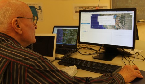
Prof. Ed Zipser of University of Utah, Flight Director for OLYMPEX, watching a flight in progress. He communicates with flight scientists via x-chat and determines the locations the aircraft will fly.
There often is an evening briefing before expected flights the following day. These are shorter and more informal than the morning briefing. However, we are expected to update the forecast narrative based on new model forecasts and current observations. Since our region of operations is the west coast, we rely heavily on satellite data over the Pacific Ocean to really understand what is going on and heading our way, so satellite interpretation skills are essential.
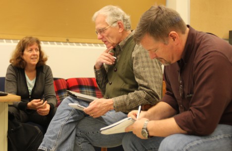
Lead OLYMPEX scientists and operations directors Dr. Lynn McMurdie, Prof. Robert A. Houze, Jr., and Dr. Walter Petersen (left to right) discuss the current situation and operation plans during a morning briefing.
Once we’re done with briefings and flights, we’re home free! But wait, there may be an early flight the next day, so it’s time to order pizza, catch a nap and be ready at 1AM. But that’s all in a day’s work for an OLYMPEX forecaster at the operations center.
Numerical weather prediction models can be run with CYGNSS data included before the satellites are even in space. This is the premise behind the Observing System Simulation Experiment, or OSSE. In an OSSE, simulated measurements from any observation platform (past, present, or future) can be assimilated into a model and their impact can then be evaluated by comparing forecasts made with and without those measurements. For an introduction to CYGNSS and how it works, please read this previous blog post.
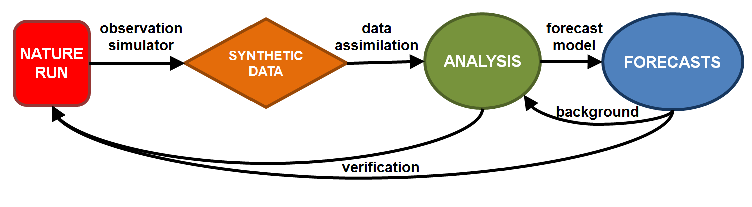
Idealized flow chart of an OSSE.
In an OSSE, the “real world” is actually high-resolution, high-quality model output from a “nature run”. That nature run is the foundation from which all observations are simulated and against which all analyses and forecasts are verified. Since the observing characteristics of instruments are known, “synthetic data” from any existing or future observation platform can be interpolated from the nature run and assigned realistic errors. If you’re living in the nature run, those synthetic data would be what your instruments would measure… including radiosondes, satellites, aircraft, buoys, and yes, even ocean surface wind speed retrievals from CYGNSS. [Note that times, dates, and events associated with the nature run are arbitrary — they do not coincide with specific events in the real world.]
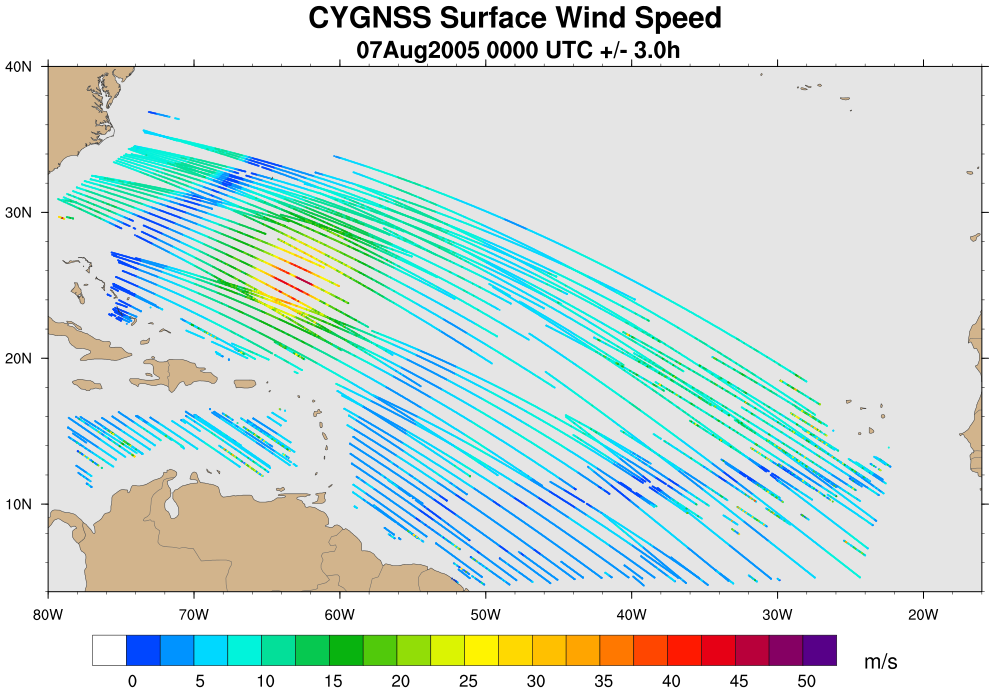
An example of synthetic CYGNSS wind speed data spanning a six hour period over the Atlantic Ocean. A hurricane can be seen north of the Lesser Antilles.
Then, the suite of observations are made available to a data assimilation (DA) system. While there are a variety of DA flavors, the basic idea is that all available observations are taken into consideration in an optimal and dynamically-consistent way to produce a best guess of the current state of the entire atmosphere. This is called the “analysis”.
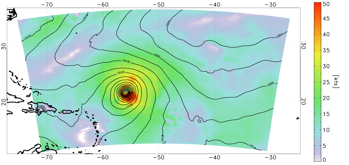
Analysis of the surface wind speed (shaded) and surface pressure (lines) on August 5 at 0000 UTC. The data assimilation method used here was a 3-D variational analysis scheme called GSI. This includes all available CYGNSS data within +/- 3 hours of the analysis time, as well as many other conventional data types.
The analysis provides the initial state for a forecast model. The forecast model, which must not be the same model used to generate the nature run, is integrated out in time. A short-term forecast (e.g. 6 hours) is used as the “background”, or first guess, for the next cycle’s analysis. Typically, the further out a forecast is run, the more it deviates from reality due to model errors, observation errors, and chaos.
The forecast model is used to produce a “control run”, which is one that includes a fixed set of observations or has a particular model configuration. Any additional data or tweaks to the DA/model system would be used to generate different runs, or experiments (“what happens if we add this”, or “what happens if we change that”). The model run is verified against the nature run by calculating errors in the analyses and forecasts — remember, the nature run is the real world in an OSSE. Output from each of the experiments can be compared to the control run to test if the errors were reduced or increased. Ideally, the addition of a new observation type such as CYGNSS improves upon the control run, but it is not always so simple in practice.
The plots below show errors in peak surface wind speed, minimum central pressure, and track for a tropical cyclone in the nature run from a control run (black line) and a single experiment with realistic CYGNSS data (red line). All of the errors from twelve forecast cycles are averaged together at the analysis time (0 hour), at 6 hours, and so on out through 120 hours. This is only an example from a single experiment, but other experiments conducted by our team include varying the DA cycling frequency, introducing “perfect” CYGNSS data interpolated directly from the nature run, adding realistic directions to the wind speeds, and assimilating higher-resolution CYGNSS data.

Errors in peak surface wind (left), minimum central pressure (middle), and track (right) for the control run (black line) and an experiment in which realistic CYGNSS data were introduced (red line). Note that lower error is ‘up’ on the y-axis on the left panel.
Based on results from a single tropical cyclone in a single nature run, simulated CYGNSS surface wind speed data do seem to have a positive impact on both analyses and short-range forecasts of tropical cyclone intensity. However, the impact on tropical cyclone track is not very noticeable, likely due to the limited influence of surface wind speeds on the storm’s steering levels.
Now we wait (im)patiently for when real data get collected and assimilated into models!
–Brian is a Senior Research Associate at the University of Miami’s Rosenstiel School of Marine and Atmospheric Science, and also blogs about hurricanes for the Washington Post.
By Christine Dow
Credit: NASA/Christine Dow
The Nansen Ice Shelf, where we have installed our GPS, is notoriously windy. This is clear from the blue ice on the surface and complete lack of snow, which gets rapidly swept away by katabatic winds (winds driven down from the glacier towards the sea by differences in pressure induced by the cold glacier air). This means that wandering around while setting up the GPS requires spikes for your shoes or else it would be like slipping around on a scalloped ice rink. To prevent the equipment from coming loose and blowing down the ice shelf into the sea, we have a set-up where wire tethers hook our solar panel and GPS box into the ice. However, it’s always encouraging to check that the systems are holding up to the elements, so we took advantage of a helicopter flight heading in that direction to check on the field equipment. It was all still there, happily recording data.
Credit: NASA/Christine Dow
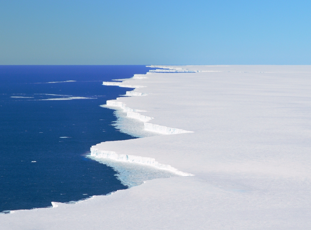
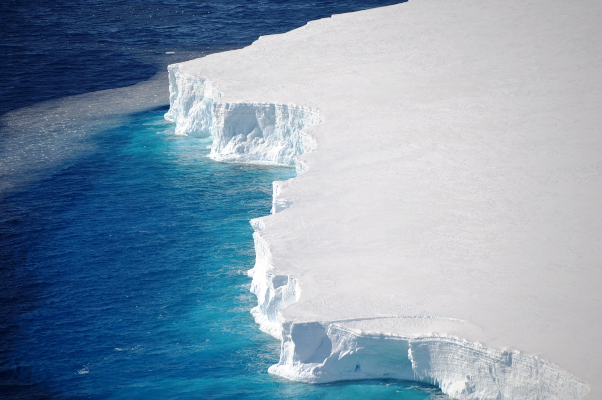
Luckily for myself and Ryan, the flight we were on was heading to the Drygalski Ice Tongue. This is a strange feature that can even be seen when looking at maps of the whole of East Antarctica. It is a floating 12 mile-wide section of ice from David glacier that sticks out 50 miles into the ocean and impacts sea ice freezing and water circulation in the bay behind it. Our approach to the ice tongue was spectacular as it headed off into the distance. At the side of the tongue, steep ice cliffs dropped into the ocean with the interaction between subsurface ice and the ocean water creating the most amazing shade of blue. We could spot groups of Adélie penguins on the remaining sections of sea ice next to the Nansen ice shelf and the Drygalski Ice Tongue.
Credit: NASA/Christine Dow
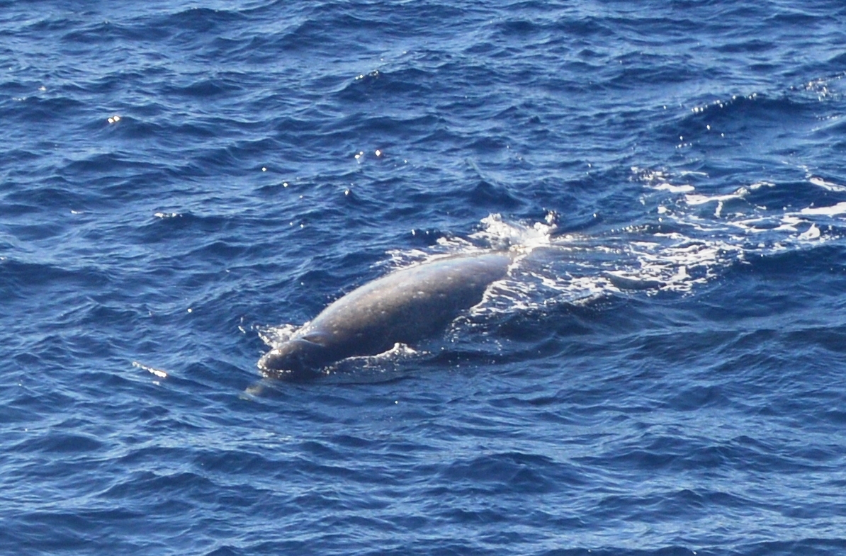
The most exciting moment was when our sharp-eyed pilot, Dom, spotted some whale spouts. We swung back around and saw four whales swimming around and breaching at the ice margin. They were Arnoux beaked whales, as we later identified, and looked nothing like any whale I have seen before – a little like very large dolphins with long pointed noses. These whales can dive for up to an hour so likely were just having a breather before heading under the ice. This was perhaps my favorite moment of the trip so far.
On the ice tongue we landed to check and download data from GPS stations that our Korean colleagues had installed several years before. We had a great view back across the bay towards Jang Bogo with Mt. Melbourne in the background. The second GPS site was fairly close to the front margin of the ice tongue and so Ryan and I had a geeky moment getting excited about being at the edge of one of the most bizarre ice features in the Antarctic.
It was a great day overall. All our stations were still standing, we saw wildlife, lots of ice and we were even back in time for a noodles and kimchi dinner.
