The global ocean is made up of five major ocean basins: the Pacific, Atlantic, Indian, Southern and Arctic Ocean. The Pacific Ocean is the largest of these basins as well as the deepest. Its expanse runs 155 million square miles and contains “more than half of the free water on earth.” Not only is it the largest and deepest ocean basin, but it is also the oldest, comprised of rocks that have been dated to be 200 million years old. You may have heard the term “Ring of Fire” associated with the Pacific Ocean. This name stems from the fact that the Pacific Ocean is prone to earthquakes and formation of submarine volcanoes along its extensive ridge and trench systems.
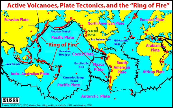
Ring of Fire
http://oceanexplorer.noaa.gov/explorations/05fire/background/volcanism/media/tectonics_world_map.html
The Pacific Ocean gained its name in the 16th century from the Portuguese navigator Ferdinand Magellan. Magellan and his crew set sail from Spain in 1519 in search of the Spice Islands located to the northeast of Indonesia. The Spice Islands were the largest producers in the world of spices such as nutmeg, cloves, and pepper. They navigated through the Atlantic Ocean and around the tip of South America after which they came across an unfamiliar ocean. He called this ocean ‘pacific’ which means peaceful. Unbeknownst to them, they still had a long journey to the Spice Islands. You can learn more about the voyage of Magellan and his crew here.
Magellan’s Voyage
http://news.bbc.co.uk/2/hi/science/nature/6170346.stm
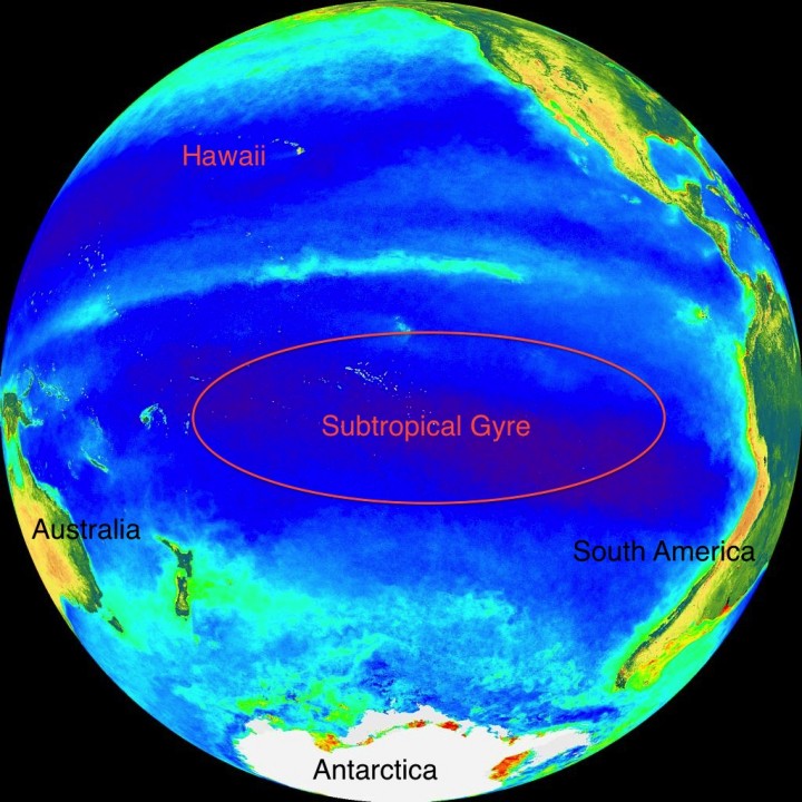
OK, back to science! The CLIVAR P16S field campaign has entered the waters of the South Pacific known as a subtropical gyre. Gyre means “circular or spiral motion.” In the ocean, wind generated surface currents travel in a circular direction, either clockwise or counterclockwise, forming a large, circular body of water. The circular direction of the currents is caused by the Coriolis Force acting to deflect motion to the right in the Northern Hemisphere and to the left in the Southern Hemisphere due to the Earth’s rotation. The South Pacific gyre is located in the Southern Hemisphere, so winds and water are deflected to the left. Because of the deflection to the left, the gyre circulates in the counterclockwise direction, forcing water to pile up in the center of the gyre. In the last post, “An Appreciation for True-Color Satellite Imagery” we discussed how microscopic plants, or phytoplankton, require nutrients to grow. Blooms (large cell numbers) of phytoplankton cannot grow in these gyres because the water that piles up within the center of circulation is nutrient deficient.
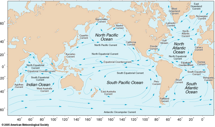
Global Ocean Circulation
http://oceanmotion.org/html/background/wind-driven-surface.htm
We can use the information about the color of the light being absorbed and reflected by the ocean to deduce the concentration of phytoplankton biomass using the proxy Chlorophyll a. Chlorophyll a is a pigment that both land plants and phytoplankton use to convert light to sugars in their chloroplast. Chlorophyll a absorbs strongly in the blue color of light. So when there is a lot of Chlorophyll a, then the light reflected back includes very little blue light. When there is very little or no Chlorophyll a, then a lot of blue light is reflected back. The figure below is an ocean color image based on the information I just described. The blue color represents little to no Chlorophyll a (or phytoplankton) present while the bright colors of yellow green and red represent increasing concentration of Chlorophyll a or phytoplankton biomass.
SeaWiFS Ocean Color image, Pacific Ocean
http://oceancolor.gsfc.nasa.gov/cgi/image_archive.cgi?c=CHLOROPHYLL
Please bear in mind that this explanation is very simplistic. You can learn more about how ocean color works here.
See the image below for the current cruise track of CLIVAR P16S. They are almost in Tahiti. Just a couple more weeks…
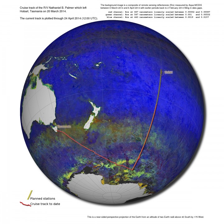
Cruise Track, CLIVAR-P16S
ACKNOWLEDGEMENTS: NASA’s Ocean Ecology Laboratory Field Support Group is participating in the US Repeat Hydrography, P16S field campaign under the auspices of the International Global Ocean Ship-Based Hydrographic Investigations Program (GO-SHIP). The US Climate Variability and Predictability Program (CLIVAR), NOAA and the NSF sponsor this campaign.

http://oceanservice.noaa.gov/facts/biggestocean.html
http://oceanservice.noaa.gov/facts/pacific.html
http://www.iol.ie/~spice/Indones.htm
http://www.rmg.co.uk/explore/sea-and-ships/facts/faqs/what-and-where-are-the-spice-islands
http://news.bbc.co.uk/2/hi/science/nature/6170346.stm
http://www.merriam-webster.com/dictionary/gyre
http://ww2010.atmos.uiuc.edu/(Gh)/guides/mtr/fw/crls.rxml
http://oceanworld.tamu.edu/students/currents/currents3.htm
http://oceancolor.gsfc.nasa.gov/cgi/image_archive.cgi?c=CHLOROPHYLL
http://oceancolor.gsfc.nasa.gov/SeaWiFS/
By Ludovic Brucker
After an unexpected phone call from the helicopter pilot on Easter Sunday, Ludo and Clem ended the second season of the Greenland aquifer campaign, with the support of Susan, Rick, Lora, Bear, the weather office, and many others. Thanks all for this Easter bunny.
We still wonder whether our campaign was successful, or fair. For sure, it was a mix of good and tough times.
The pluses, making our campaign a good time:
– We’re back from our field site, healthy and with all our fingers and toes!
– We set up an almost perfect camp, limiting drift considerably.
– Our two tents survived 65-knot winds!
– We had saucisson (dry cured sausage), and cheese for fondue!
– No polar bear smelled our food!
– We collected over 17 miles (28 kilometers) of high-frequency (400 MHz) radar data, including 12 mi (20 km) in one day (equivalent to half a marathon!)
– Along a 1.24-mi (2-km) segment of the 2011 Arctic Circle Traverse, we deployed 5 radars operating at 400, 200, 40, 10, and 5 MHz.
– We installed an intelligent weather station developed by the group at IMAU, in the Netherlands.
– We drilled down to 28 feet (8.5 meters) to record the density and stratigraphy of the ice layers.
– We have GPS taken positions during a week, which will help us calculate the velocity and flow direction of the ice in this basin.
The minuses, making our campaign “different”:
– Ten days of weather delays before the put-in flight to our ice camp location.
– Rick could not make it to the field with us.
– We never had three consecutive half days with weather suitable for work.
– Getting a sore throat from shouting to hear each other less than a meter apart.
– During the one day of great weather, we tried to drive down a pilot tube to install a piezometer in the aquifer. This technique is adapted for ground water found within rocky soils. It was the first attempt to do it in the Greenland firn. Driving the metal pipes in the snow through the ice layers was a nightmare, we had to pound on those pipes really hard to make them go through the thick ice layers and we ended up breaking them. At one point, we thought it was broken slightly deeper than 6 ft below the surface, so we dug a pit down to fix it. Well, it turned out that the broken piece was actually 13 ft down — we spent the only full day of great weather breaking our equipment.
– We ran out of cheese for fondue, and of saucisson.
– Sunscreen was completely useless this season.
The “funny” stuff:
– 30 m/s wind is brutal, though not necessarily hilarious.
– High-wind speed does not make the clock spin faster, only the anemometer.
– Supporting text messages and jokes from our family, colleagues, and office mates.
– Attempting a radar survey with a sled taking off every other gusts.
– Calling the Met Office for a weather forecast: “Hello! Since it’s windy here we are wondering what will happen in the next 36 hours.” “Yes, I can confirm that you are experiencing wind.” “Thanks so much for the confirmation, but there was no room for doubt.” “Oh, but it’s a nice spike on the computer screen! It won’t blow more, but it won’t stop soon. Be careful out there”. Patience with Mother Nature is the #1 fundamental.
– Coastal storms from the East might be our favorite storms on the ice sheet: wind stops, and temperatures increase, but it snows, snows, and snows.
– Sixteen feet of seasonal snow is deep, especially with the top 2 feet of fresh snow becoming harder and harder as they it gets compacted by the wind.
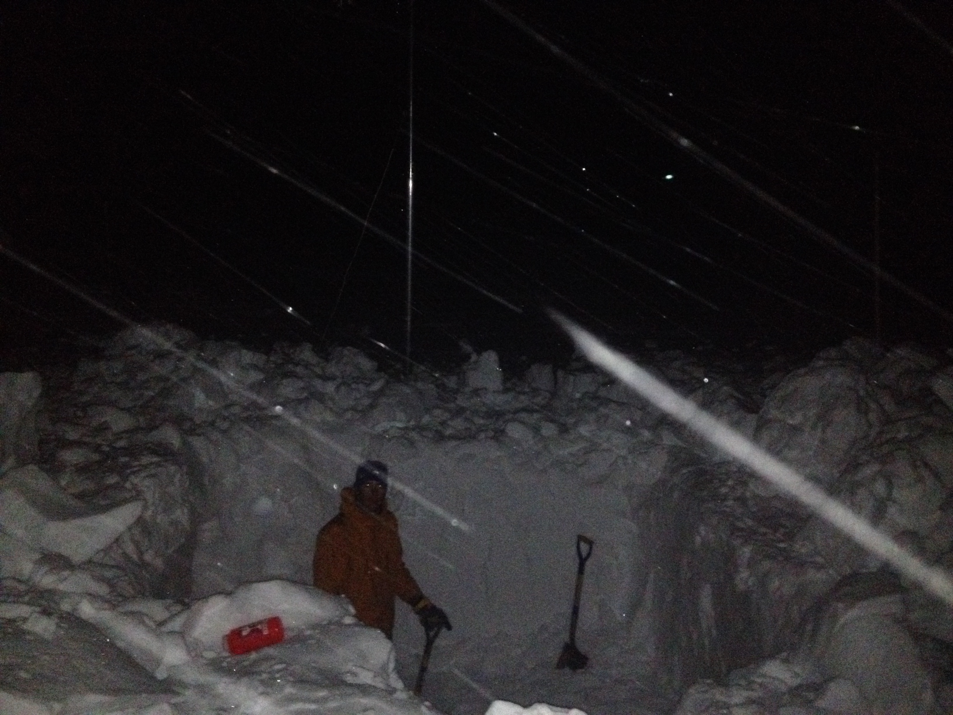
– Excavating 1765 cubic feet of snow between 8pm and 11:30pm (you got to use the weather window whenever you have it.)
– The frost all around our sleeping-bag head every morning.
– The 40 hours laying down in the sleeping bag.
– The melody of the wind on our tents and through the bamboo sticks we stuck around them.
– Using the sleeping bag to store hats, balaclavas, gloves, socks, boot insulation, contact lenses, tooth paste, sun screen (it was nice to dream about the day we would need it), batteries, head lamp, snacks, water bottles (ideally liquid and not spilling.)
– The pilot phone call at 8 am on Easter Sunday: “Good morning, happy Easter! Don’t go for a ski strip today, we will come pick you up in 3-4 hours!”
This was the synopsis of our 13-day adventure on the ice sheet. Even though we have been pulled out from the ice sheet, we still have some work to do, such as cleaning and drying our cargo and repackaging it for shipping to either Kanger, or the US.
Now, we would like you to enjoy some photos taken in the field. Thanks again for spending some times reading the blog and following us! Until the next campaign, enjoy each season and stay warm! As we say in French: “En Mai, fait ce qu’il te plaît!” In English, it translates to something like: “In May, do as you please!”. Yup, we’re heading back to the office and will hide behind a computer screen for the months to come.
All the best,
Ludo & Clem
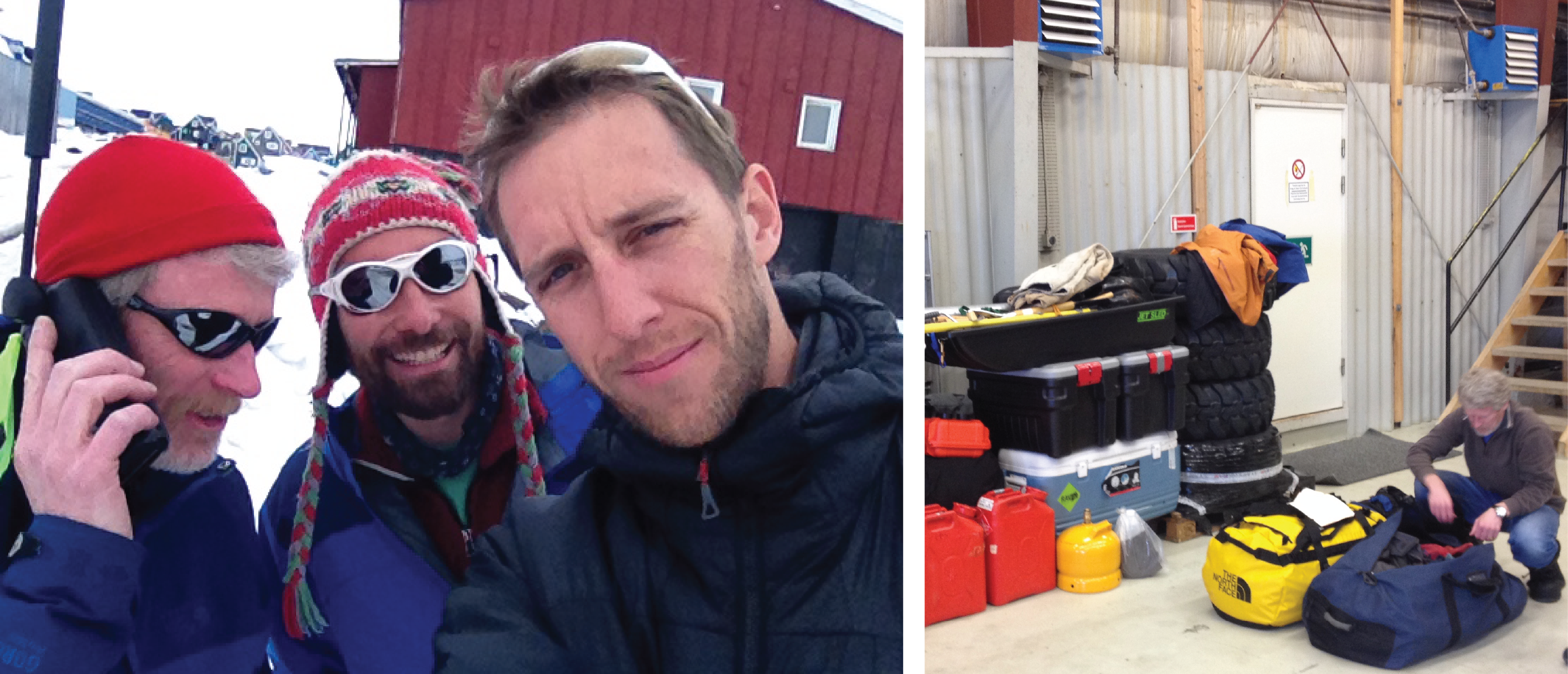
(Left) As weather-delay days continue to keep us in town, Rick calls the weather office to assess whether we can afford to spend more days waiting to be deployed on the ice sheet. (Right) The saddest moment of our campaign, when Rick had to remove his gear from our cargo because he wasn’t coming with us to the field.

(Left) At the Tasiilaq heliport, Ludo waits for our put-in flight on the cargo. (Right) The Air Greenland B-212 helicopter with blue skies and high clouds. After 12 days of patiently waiting, it looks like it’s a go!
Flying over the sea-ice covered Sermilik fjord to reach the ice sheet.

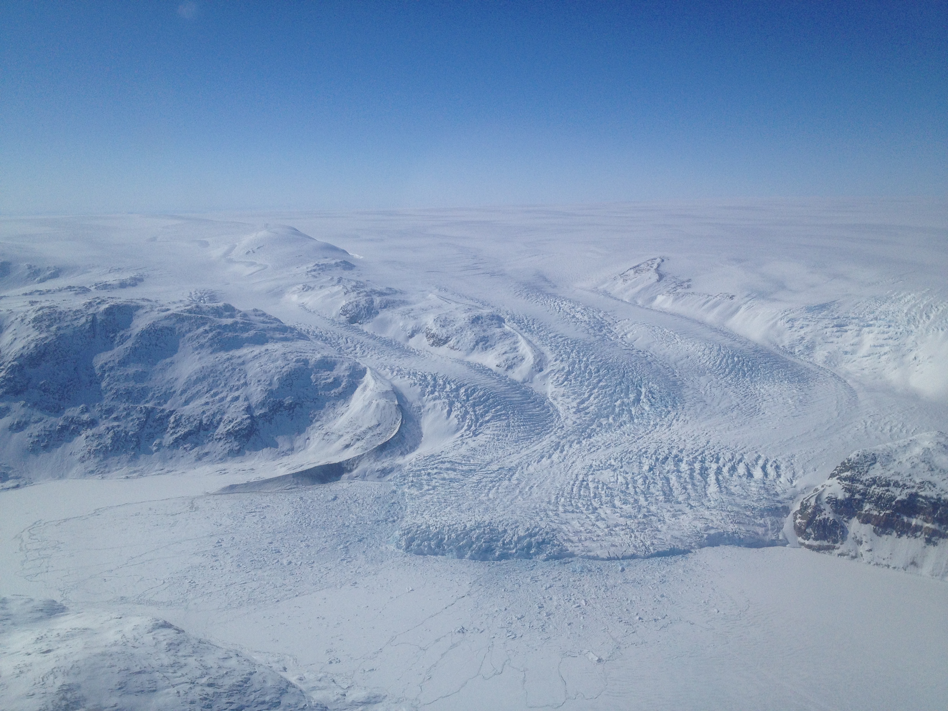
Getting closer to the ice sheet, flying over crevassed tributary glaciers.
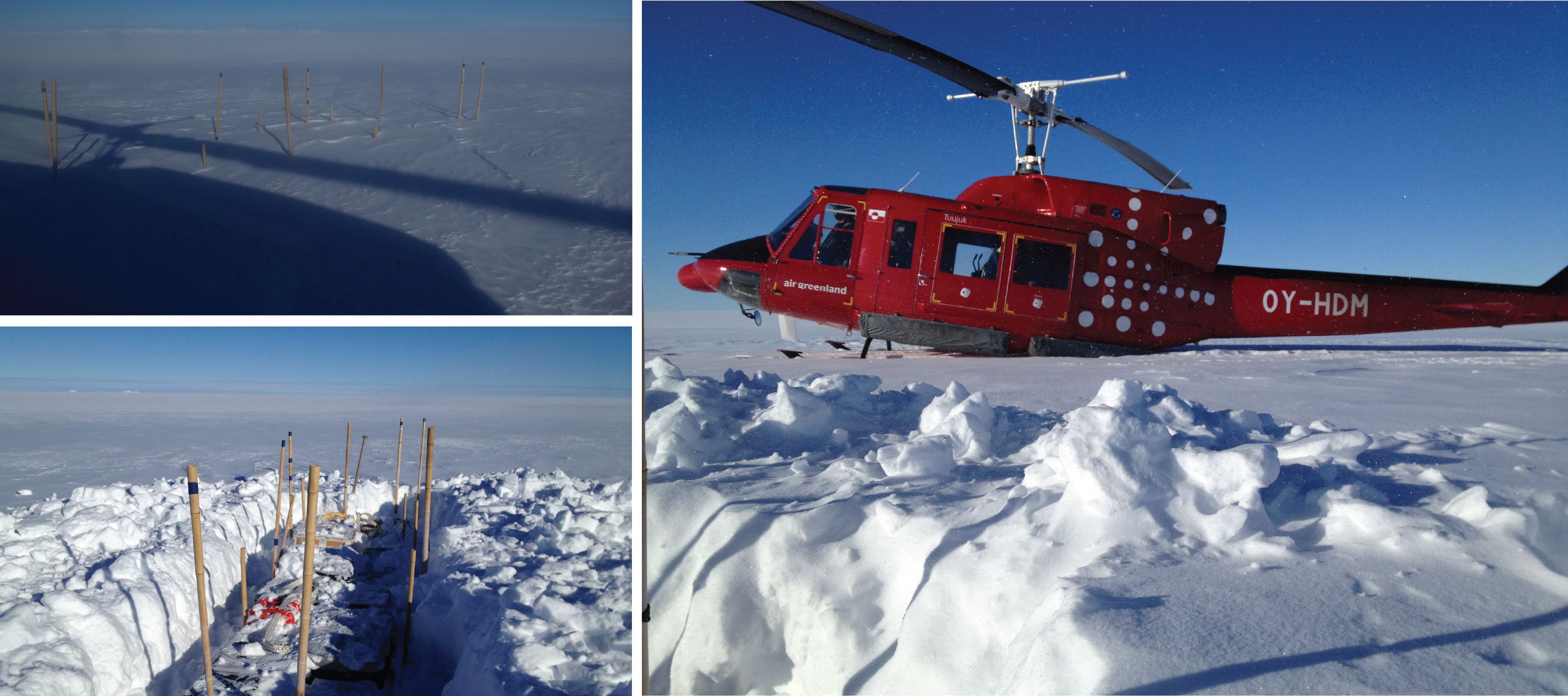
(Left) Our cargo, dropped almost two weeks ago, got buried under 2 feet of snow. But all the pieces were there! (Right) The B-212 landed near our cargo for a final move to the ice camp location.
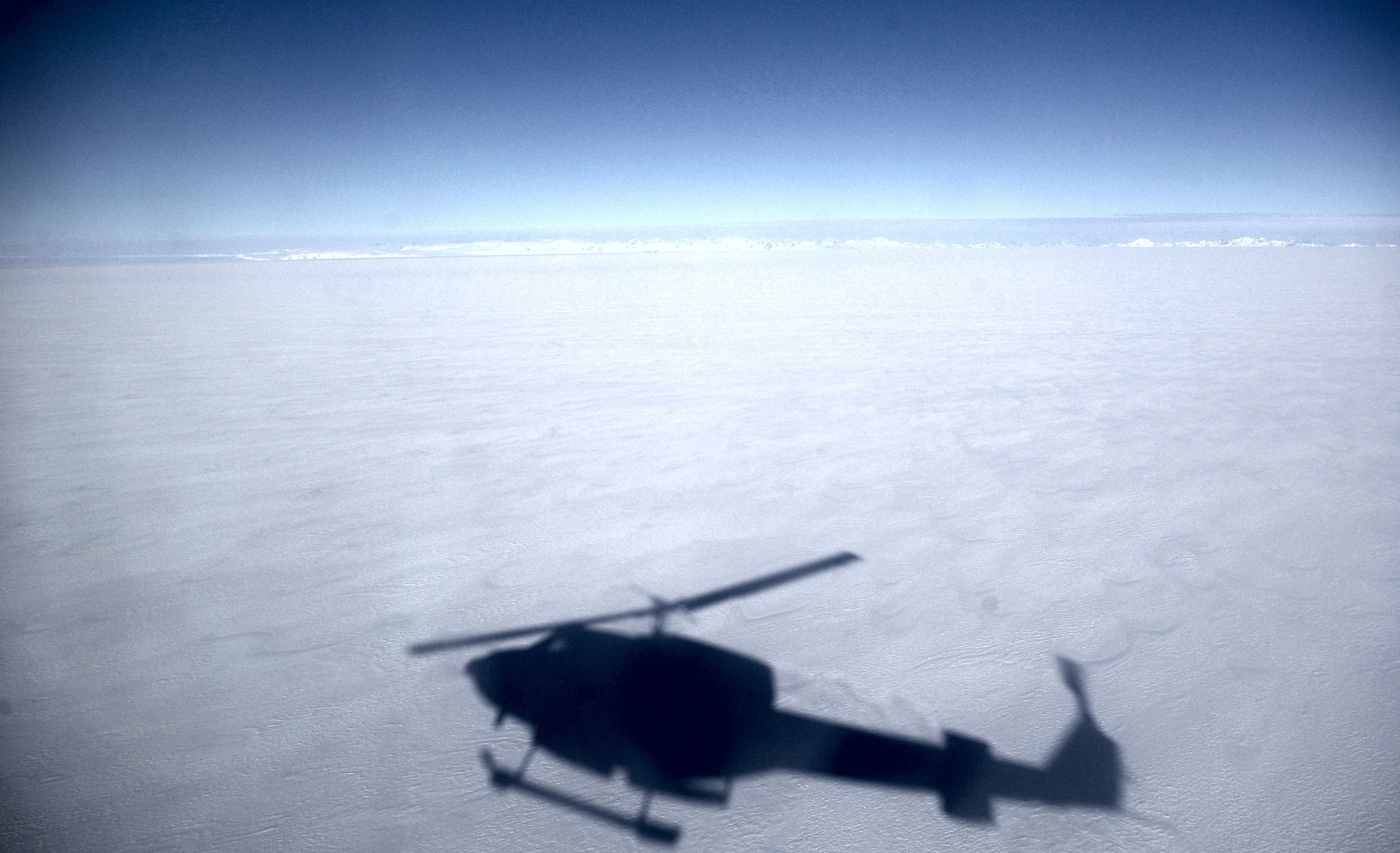
Approaching our camp site.
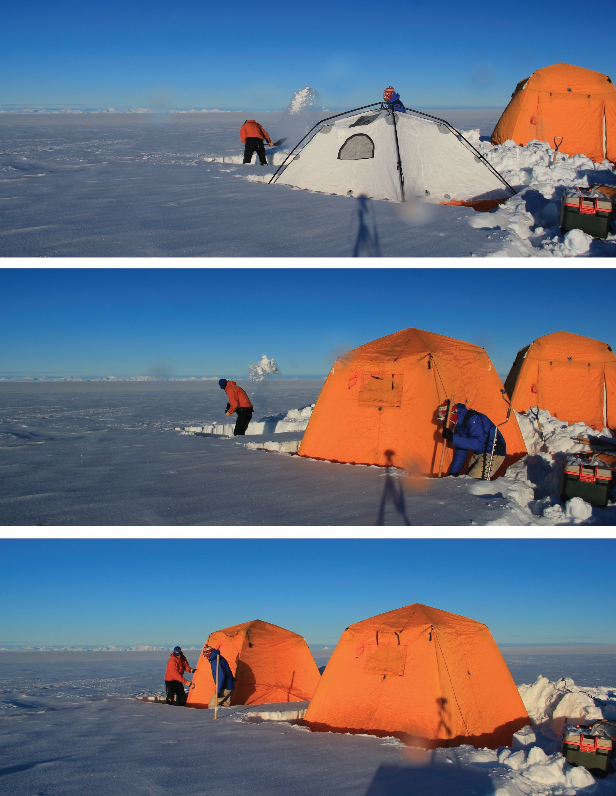
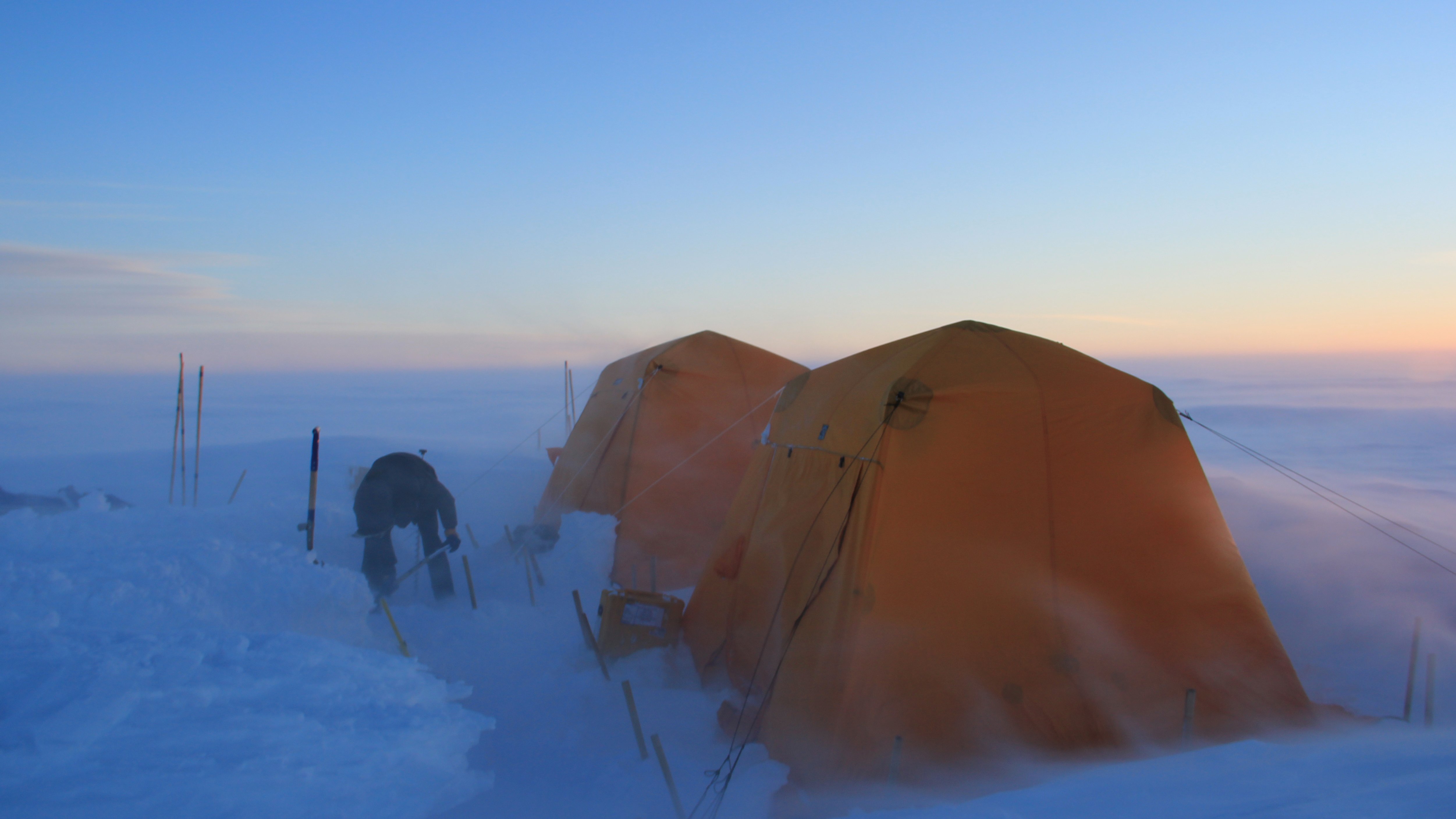
Minutes after the B-212 had left Clem and me on the ice sheet, we were already shoveling the fresh snow to install our cooking and sleeping tents before dark. This was no time for play, this was no time for fun, there was work to be done.
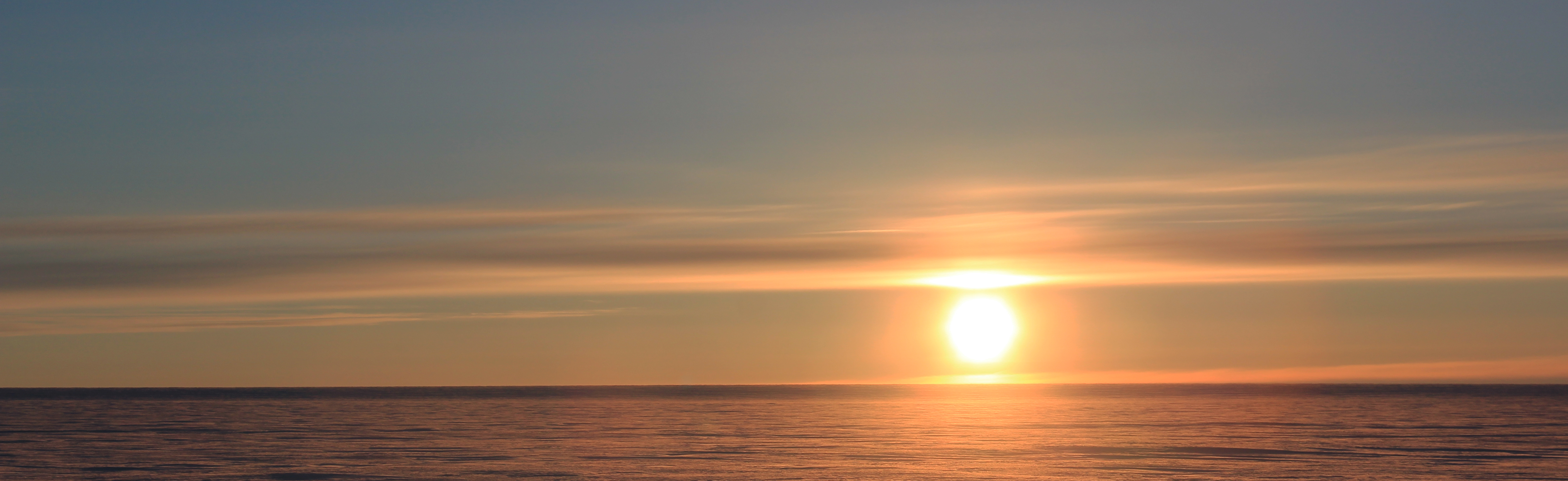
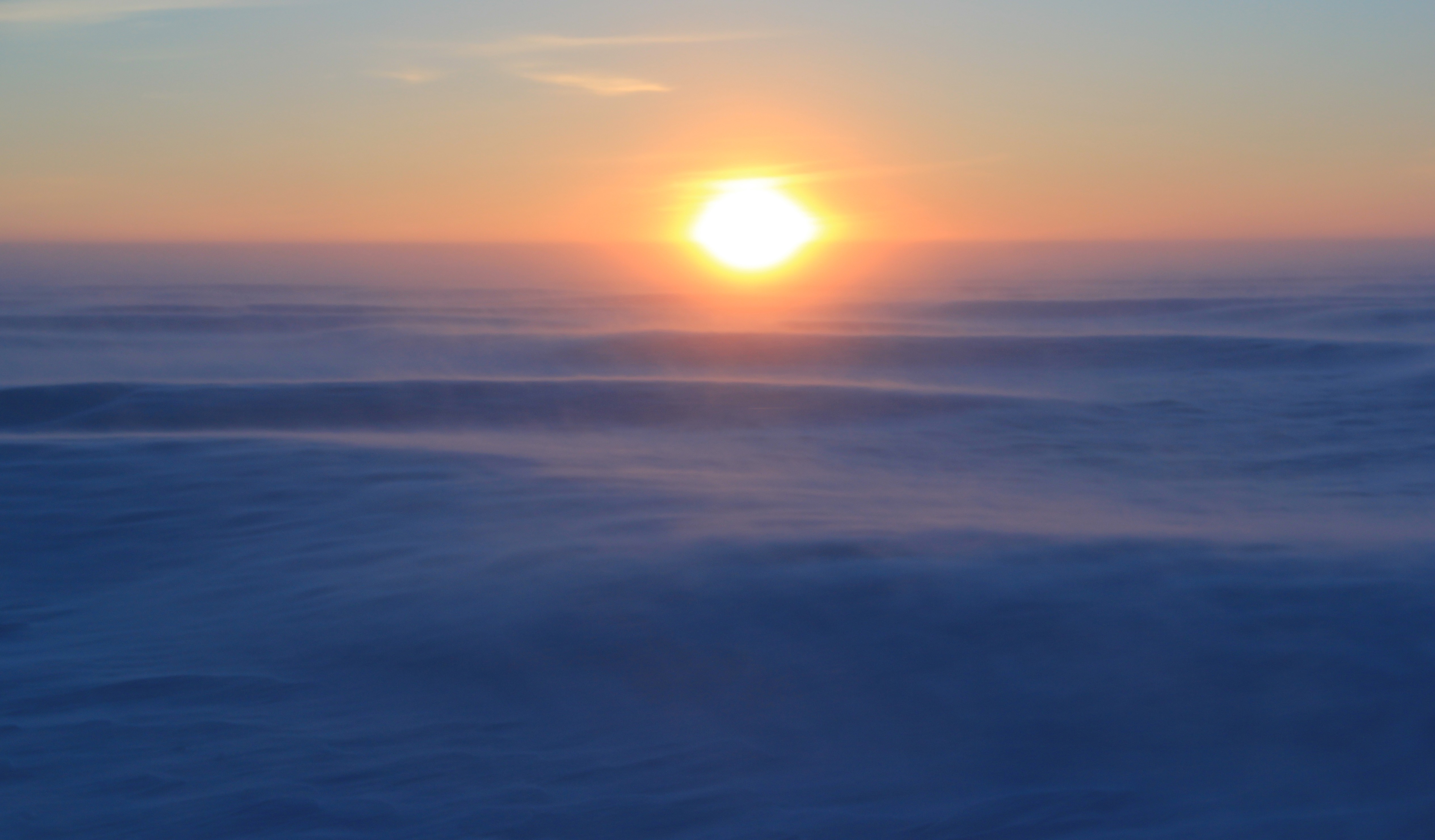
Our first pretty sunset in Greenland. In one month, we saw two of them.

Early morning selfie! Not fully ready yet to put our cold weather gear on.
Shoveling, a typical activity at camp. Luckily this year we did not have to shovel too much to maintain our tents.
With the amount of fresh snow and the katabatic winds increasing, snow dunes were forming perpendicular to the direction of the wind — it was like being at sea! Half a day later, sastrugis developed along the wind direction and snow became hard and compact.
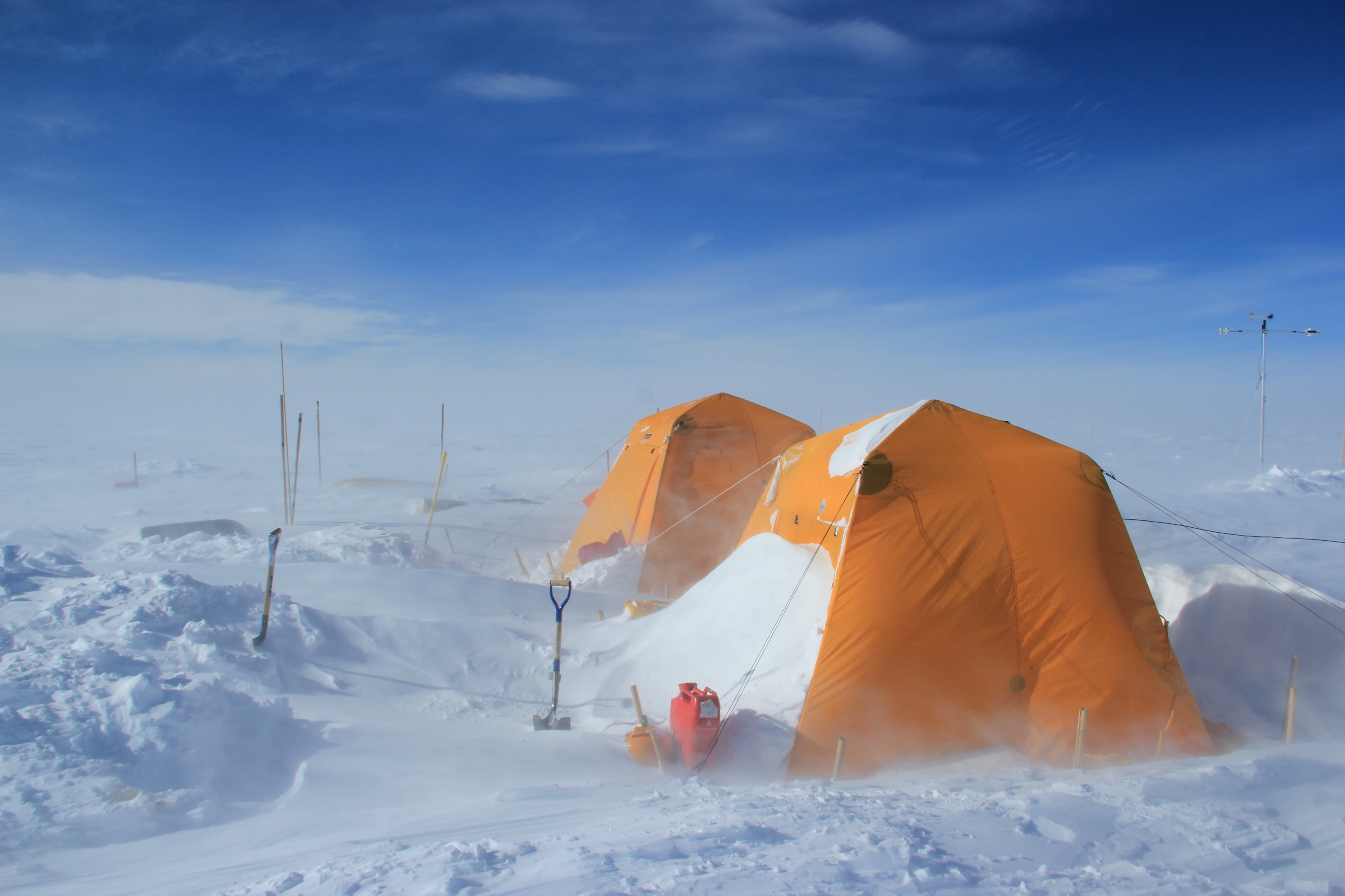
A snow drift blocking the door of the kitchen tent.
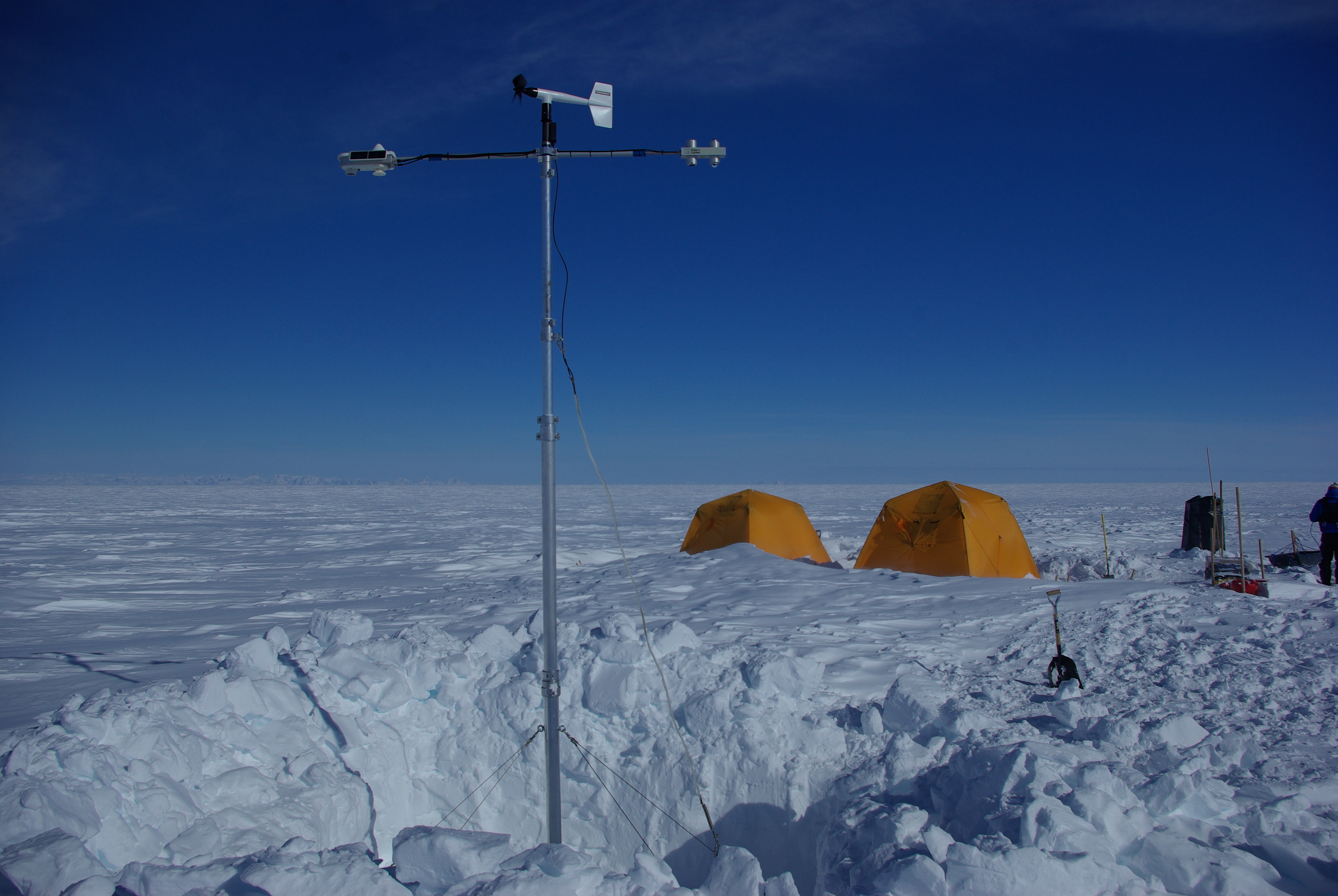
The IMAU intelligent Weather Station, installed in its snow pit before we refilled it.
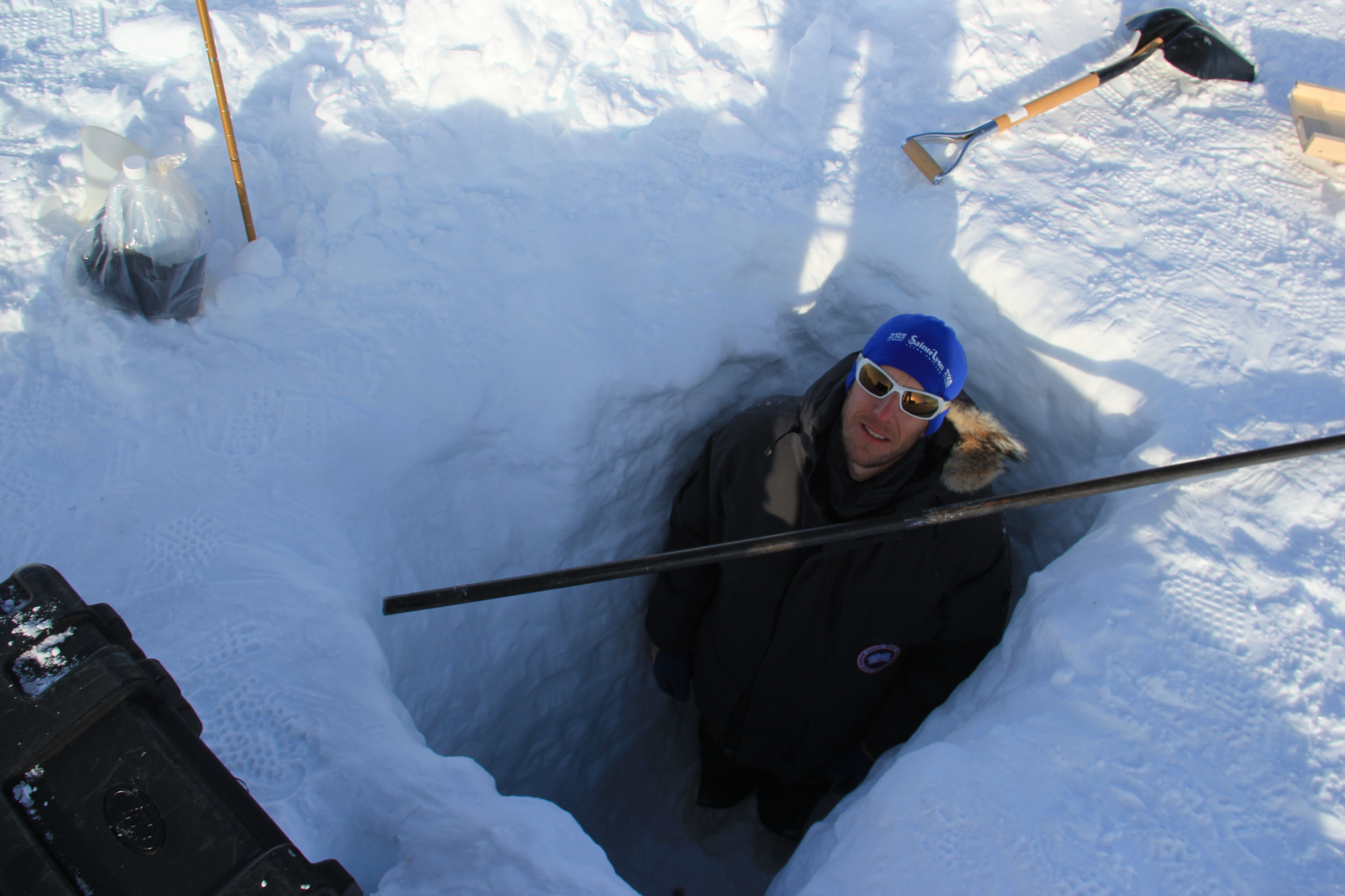
Ludo inside a 2-m-deep pit dug with the hope to repair a broken pilot pipe for installing a pressure transducer in the aquifer.
Ludo, inside a larger 2-meter-deep pit dug after dinner with easterly winds increasing as another coastal storm was coming bringing more snow. Our rationale was that the sooner we dug, the less snow we’d have to remove.

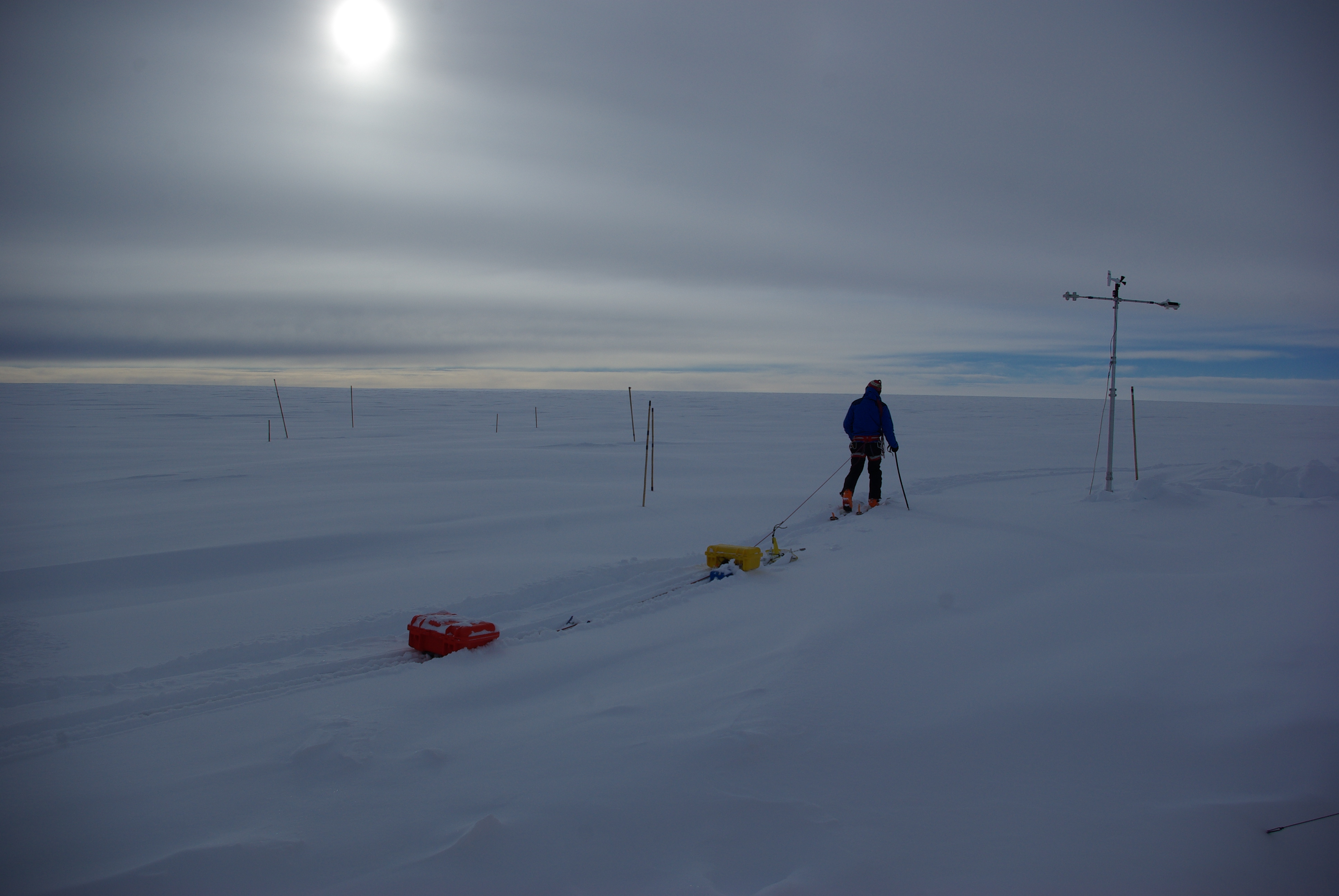
Two hours before being pulled out from the field, Clem was dragging the 200 MHz radar, and carrying a GPS unit.

(Left) Snow accumulated on our tent entrance overnight. We monitored it carefully every half hours from 2 am to the late evening. We took care of it a couple of times! (Middle) Clem calling the weather service to find out what wind speeds would hit us during the night. (Right) Our last saucisson, hanging over the snow/water pot.
Clem uses an evening break in the weather to drag a low-frequency radar in the fresh snow deposited in the previous hours.
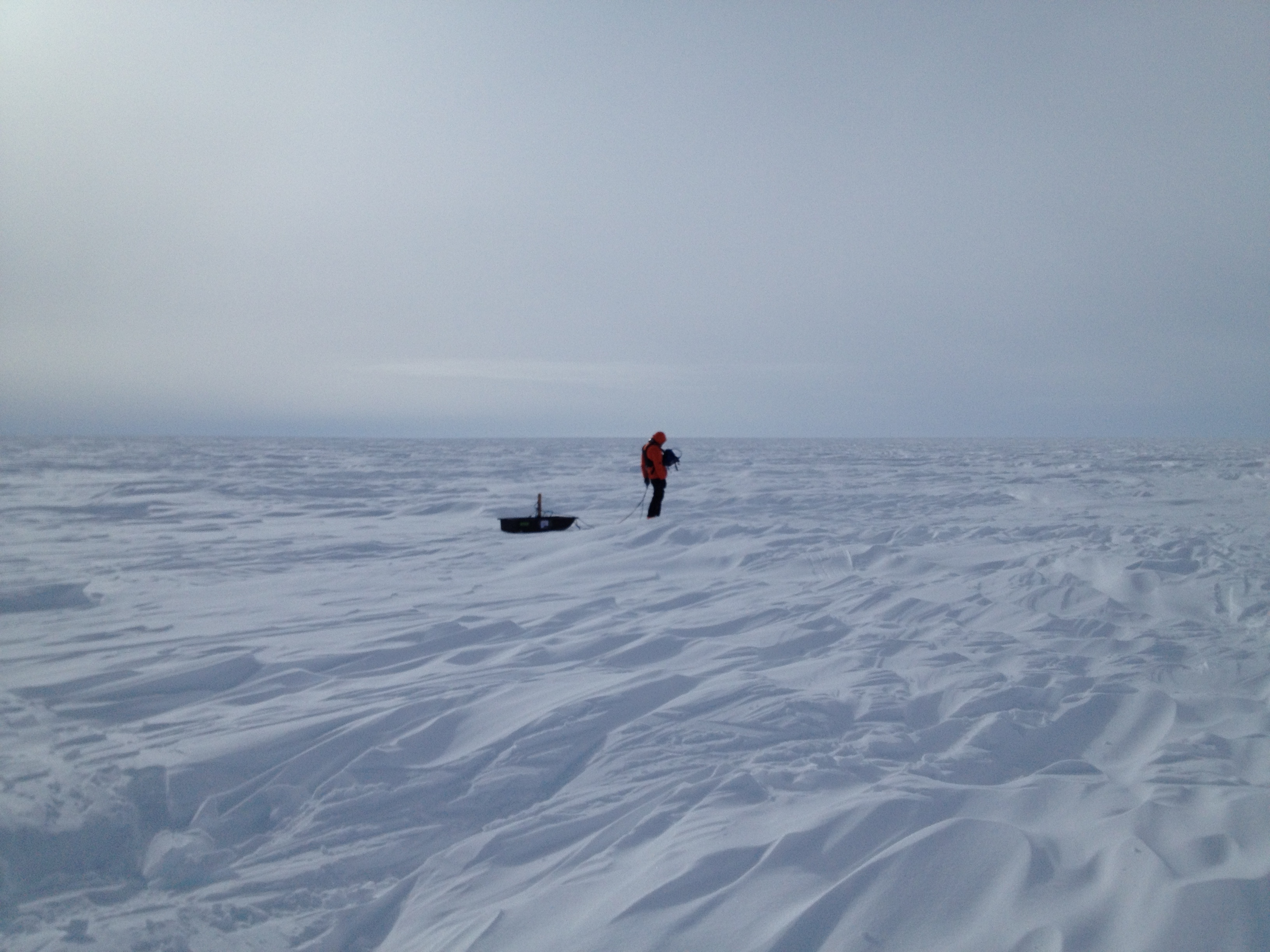
Clem dragging the 400 MHz radar over the sastrugis, a challenging surface to work with.
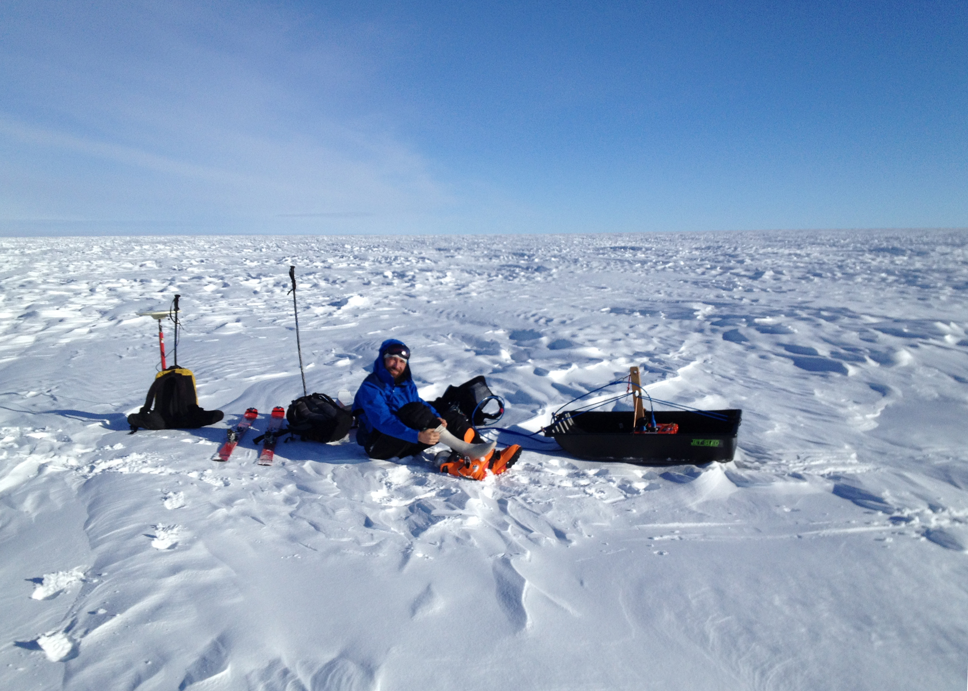
Weather was clement enough with Clément to allow him for a pit stop during our half-marathon radar day around camp.

A new day, different weather, and another attempt to collect more radar data. Since we aimed at collecting surface-based radar data, not airborne radar data, we quickly had to stop because the wind would make the radar system take off with every other gust.

Pictures taken just one hour apart. In the top one, we were setting up a radar system. In the bottom one, we were actively wrapping it due to sudden katabatic winds that picked up in less than 10 minutes.
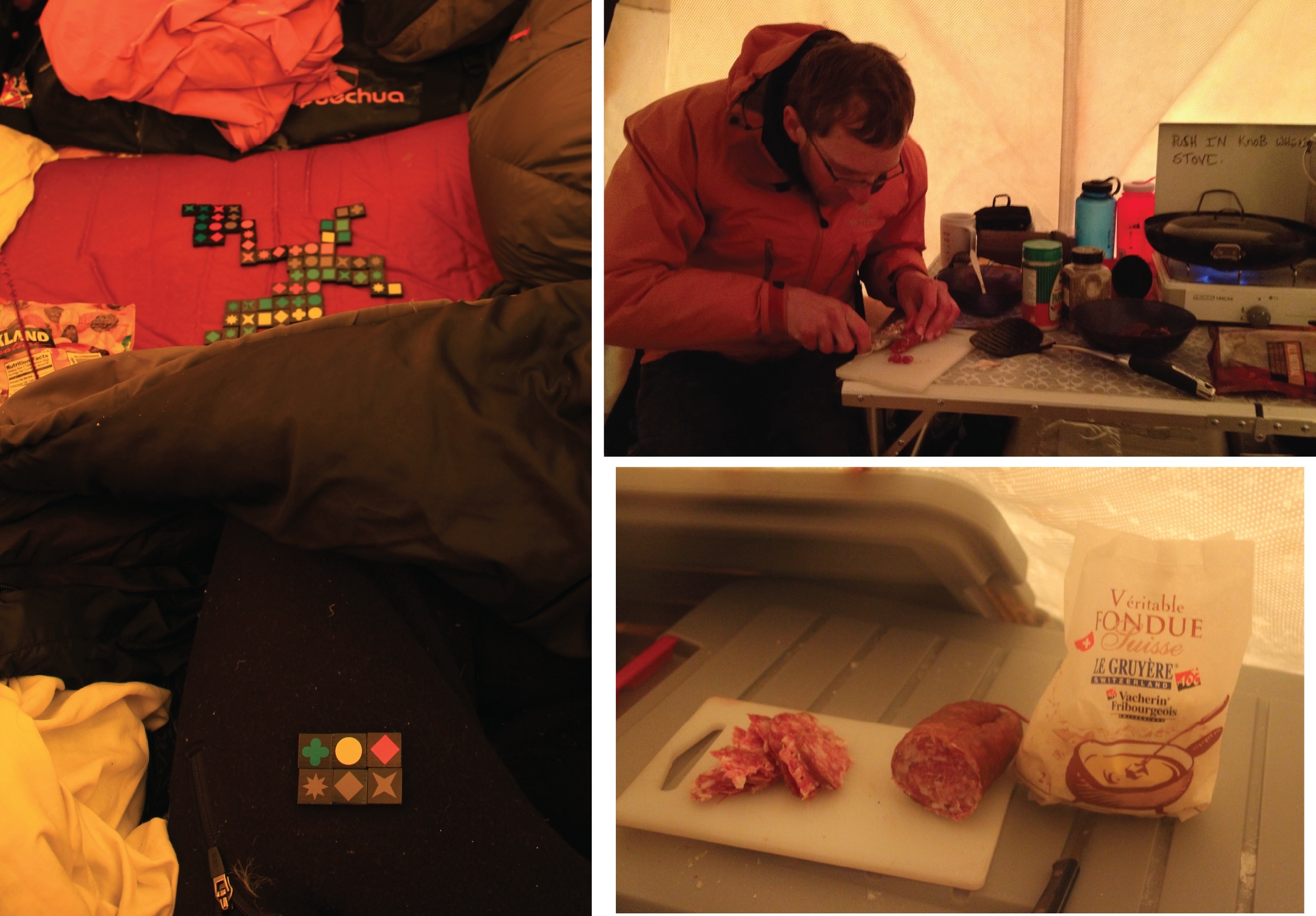
Indoor activities while the winds prevented us from working. (Left) Playing domino with mitts in a shaking tent, unforgettable times! (Right) Good food to keep us happy. Merci maman for thinking about us before leaving home.

Our flight back had already been canceled twice. It turned out that this was our last evening at camp. We had a total of two pretty sunsets: one on the first day and the second 12 days later, on our last evening.

Our bags, ready for a surprise pull-out flight! Happy Easter!

A great moment: the landing of the B-212. We were being pulled out!

The crew and Ludo finish up loading the B-212.
Last view of the ice sheet and glaciers.

Forty minutes after leaving our camp, we see signs of life: a view of Tasiilaq (top) and Kulusuk (bottom), minutes before landing.
We’d like to finish with this quote from the French explorer Jean-Baptiste Charcot, who led the second French expedition in Antarctica around 1910:
“D’où vient l’étrange attirance de ces régions polaires, si puissantes, si tenaces, qu’après en être revenu ou oublie les fatigues, morales et physiques, pour ne songer qu’à retourner vers elles? D’où vient le charme inouï de ces contrées pourtant désertes et terrifiantes?” (“Where does the strange attraction of the polar regions come from, so powerful, so stubborn, that after returning from them we forget the fatigue, moral and physical, only to think of returning there? Where does the incredible charm of these lands come from, however deserted and terrifying?”) Jean-Baptiste Charcot, Le Pourquoi Pas?
We have spent the last few weeks discussing the differences between inherent and apparent optical properties in the ocean and how we measure them. Now let’s take a moment to appreciate the information these data give us. I am sure many of you have seen satellite images of the ocean, hurricanes, etc. on the news and at other outlets. A lot of work goes into each and every one of those images and they can show remarkable things on a global scale that would be difficult to detect through fieldwork alone.
Below you will see a true color image of a phytoplankton bloom in the Barents Sea that was acquired on August 24, 2012 by NASA’s MODIS Aqua satellite . The Barents Sea is part of the Arctic Ocean and is located off the northern coasts of Norway and Russia. The word phytoplankton is Latin for plant (phyto) and to wander or drift (plankton). Phytoplankton can photosynthesize and produce energy from sunlight just like plants do on land. They also take up carbon dioxide and release oxygen like land plants. Phytoplankton are an important component of the food chain as other organisms such as zooplankton and fish use them as a food source. Additionally, they play an important role in the global carbon budget because they can use the carbon (CO2) that is absorbed by the ocean to make sugars.
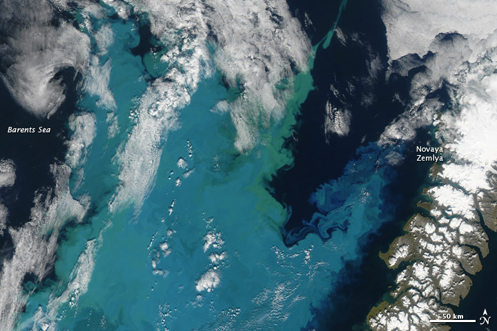
Barents Sea phytoplankton Bloom
There are many types of phytoplankton that bloom in the ocean including diatoms, dinoflagellates, and coccolithophores, just to name a few. You can learn more about different phytoplankton groups here. They all rely on specific nutrients, such as nitrogen (NO3, NO2, etc.), phosphorous (PO4, etc.) and trace metals (iron, magnesium, etc.). Phytoplankton blooms occur when many individuals, or cells, of one species are present in one region of a body of water (lake, estuary, open ocean), altering the color of the water. In the image above, the water is dominated by a species of coccolithophore. Coccolithophores are a type of phytoplankton that are covered with plates made of calcite called coccoliths. Calcite, or calcium carbonate, is white giving that creamy white look to the water. You can learn more about this coccolithophore bloom here.
This next image was recently featured on NASA’s OceanColor website. It was taken off the western coast of Africa where a current called the Benguela current flows northward bringing water from the South Atlantic and Indian Ocean. In this image from April 10, 2014 we can see a yellow discoloration in the water. I just learned that this area is prone to toxic hydrogen sulfide precipitation events that have been known to cause fish and other marine animal mortalities. Amazingly, these events have been captured using satellite imagery. However, the cause of this particular discoloration has not, as of this post, been determined. This is where fieldwork comes in! Still, it is very cool! Thanks to Norman Kuring at NASA Goddard for locating this feature.

Discoloration in the Benguela Current off the coast of Namibia
You can enjoy many other satellite images at NASA’s Visible Earth website.
References:
http://www.worldatlas.com/aatlas/infopage/barentssea.htm
http://earthobservatory.nasa.gov/Features/Phytoplankton/
http://www.bigelow.org/foodweb/microbe0.html
http://protozoa.uga.edu/portal/coccolithophores.html
http://oceancolor.gsfc.nasa.gov/
http://oceancurrents.rsmas.miami.edu/atlantic/benguela.html
http://oceancolor.gsfc.nasa.gov/cgi/image_archive.cgi?i=423
http://www.sciencedirect.com/science/article/pii/S0967063703001754
ACKNOWLEDGEMENTS: NASA’s Ocean Ecology Laboratory Field Support Group is participating in the US Repeat Hydrography, P16S field campaign under the auspices of the International Global Ocean Ship-Based Hydrographic Investigations Program (GO-SHIP). The US Climate Variability and Predictability Program (CLIVAR), NOAA and the NSF sponsor this campaign.

By Rick Forster
Our team finally made it to the ice sheet on April 8, after being delayed for almost two weeks due a series of storms. That day, we awoke to patches of blue sky over the village of Tasiilaq and were eager to get to the heliport for our scheduled 11:40 AM flight to the ice sheet. Lingering clouds over the ice sheet delayed our departure about three hours.

The village of Tasiilaq on the day of our flight to the ice sheet in SE Greenland where the Air Greenland B-212 helicopter is based. (Credit: Rick Forster.)
Once we saw the Air Greenland helicopter returning from its last trip to the local settlements for the day, we knew our flight was next. The trip to our research site on the ice sheet takes about 30 minutes.
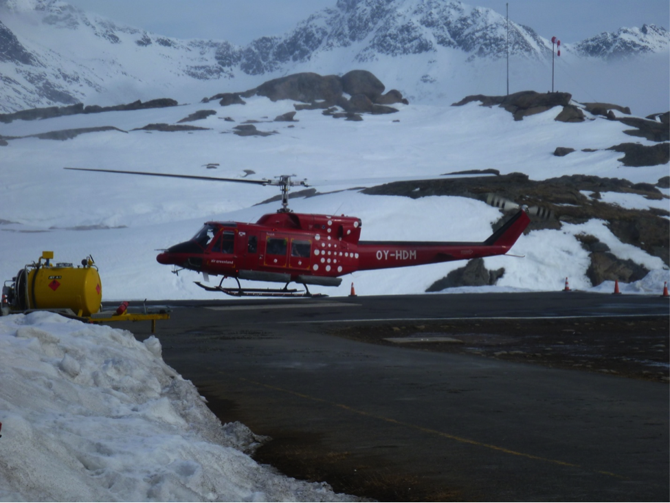
The Air Greenland B-212 helicopter landing in Tasiilaq. (credit: Rick Forster.)
The two-week weather delay meant I had to return to the University of Utah while Clem and Ludo would stay on the ice sheet for about 10 days to gather data and perform experiments on the Greenland aquifer. It was a hard decision to make, but I had commitments and if I stayed with the team on the ice sheet, we would all have to leave before all the science could be completed. Ludo and Clem’s schedules were more flexible so they will be able to extend their trip to spend extra time on the ice. I went with the team to the ice sheet to help unload the camp gear from the helicopter at the research site.
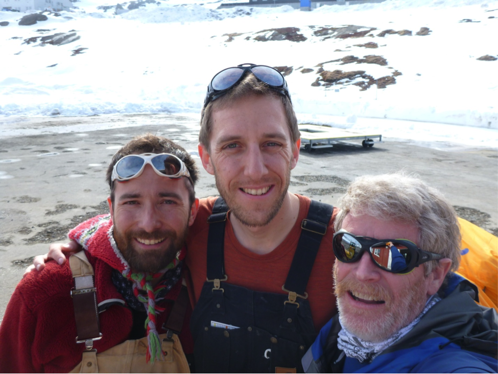
From left to right: Clément Miège, Ludovic Brucker, and Rick Forster happy to be finally boarding the helicopter for the flight to the ice sheet. (Credit: Rick Forster.)
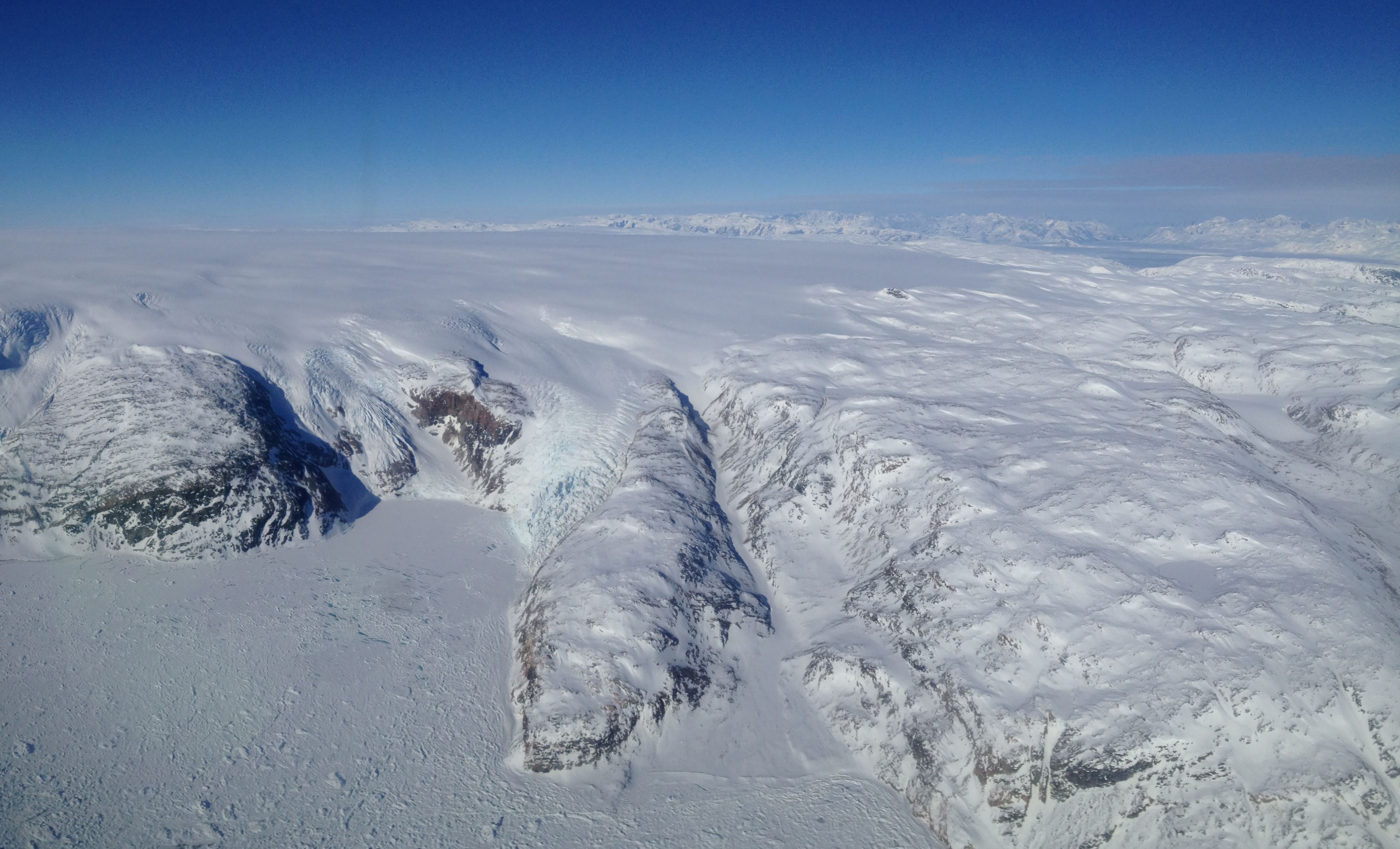
The flight to the site was spectacular, going over sea ice chocked fjords and outlet glaciers draining the ice sheet.

An outlet glacier draining the Greenland ice sheet into an ice covered fjord. The individual rough blocks of ice within the smooth surface of the frozen fjord are icebergs that calved off the glacier last summer and are now trapped in the winter fjord ice. (Credit: Rick Forster.)
Once at the research site, our team, including the pilot and flight engineer, quickly unloaded the cargo from the helicopter. The heaviest gear could be left closer to the helicopter, while the lighter pieces needed to be dragged farther away and held down by Ludo and Clem to keep them from being blown away from the winds generated by the helicopter taking off. The ice sheet surface was smooth and soft with knee-deep powder, great for skiing but not so good for moving cargo and setting up camp.
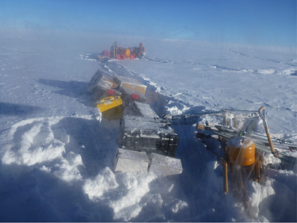
Clem, Ludo, and the science and camp cargo waiting for the helicopter to take off. (Credit: Rick Forster.)
Clem and Ludo will spend the next week and half gathering additional data on the Greenland aquifer from a variety of ice penetrating radar systems and installing an automated weather station for our colleagues at Institute for Marine and Atmospheric research Utrecht.
One of the greatest tools used by oceanographers today for measuring ocean processes is the CTD. CTD stands for Conductivity, Temperature and Depth. Conductivity is a measure of ocean salinity. The CTD is used to collect profile data in the ocean. The CTD is typically accompanied by a carousel, or rosette, of large bottles (Niskins) that can hold about 10 liters (2.6 U.S. gallons) of water. Some Niskins are large enough to hold 30 liters. These bottles have spring-loaded caps that can be triggered to close at specified depths. The CTD and other sensors, such as a chlorophyll fluorometer, and an Acoustic Doppler Current Profiler (ADCP) that measures current velocities, and other sensors can also be attached within the rosette package.
The whole package is connected to a very long cable and is mechanically lowered by a winch operator down through the water column, which is called the ‘downcast.’ During the downcast, information about salinity, temperature, depth and data from the other sensors are sent to a computer on board the ship. The computer is connected through the cable that is lowering the package. The downcast is halted once the package reaches close to the ocean floor. When the CTD is raised back to the surface, the ‘upcast’, each of the Niskin bottles is closed at assigned depths, collecting water as it travels back to the surface.
Once the Rosette package is back aboard the ship, the scientists are able to collect water from the bottles for their analyses. The parameters collected and analyzed during CLIVAR campaigns includes but are not limited to: salinity, oxygen, nutrients, chlorofluorocarbons (CFCs), dissolved inorganic carbon (DIC), total alkalinity, pH, dissolved organic carbon (DOC), helium, and tritium.
Certain compounds, such as some radionuclide (tritium, carbon-14, etc.) and CFCs, can be used as ‘tracers’. These tracers are used to follow ocean currents and calculate the age of water parcels. CFCs were prominently used in refrigerators and air conditioning units until the 1970s when they were banned over the concern of ozone depletion. You can learn more about the CFC tracer program here. Through the WOCE and CLIVAR programs CFC concentrations have been measured all over the world.
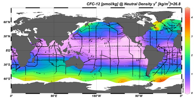
Map of global CFC measurements
http://www.pmel.noaa.gov/cfc/
The measurement of pH, total alkalinity and DIC are important for monitoring ocean acidification. Ocean acidification (OA) is the decrease in ocean pH as a result of an increase in carbon dioxide (CO2) absorption by seawater. OA is a prominent concern in today’s world. CO2 is pumped into the atmosphere from everyday human activities, such as emissions from vehicles and industrial pollution. Each year approximately 25% of the CO2 pumped into the atmosphere is absorbed by the ocean. Although plants can use CO2 for photosynthesis, the increase also has negative implications. As the amount of CO2 absorbed by the increases, the pH is expected to continue decreasing.
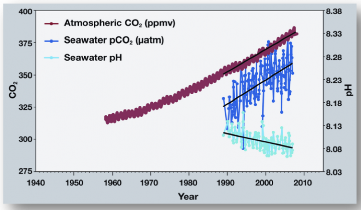
pH time series
http://www.pmel.noaa.gov/co2/story/OA+Observations+and+Data
The pH of the ocean directly affects organisms that form calcium carbonate shells or structures, like corals, oysters, clams and sea urchins. An acidic environment causes the calcium carbonate to dissolve and makes it more difficult for the organisms to make their calcium carbonate skeletons. Therefore, it is important that programs like CLIVAR are monitoring global CO2 concentrations (part of the DIC pool), total alkalinity (the ability for the ocean to neutralize acids) and pH. We know that decreases in ocean pH can negatively impact marine organisms. You can see more about the effect of ocean acidification or marine organisms here.
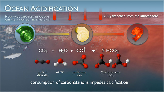
Ocean Acidification
http://www.pmel.noaa.gov/co2/story/What+is+Ocean+Acidification%3F
As I was conducting some research for this blog post I came across this article that was posted at the Earth Observatory in 2008 about the global carbon budget. I thought it was appropriate to bring it back here.
Earth Observatory article from 2008
References:
http://www.whoi.edu/home/oceanus_images/ries/calcification.html
http://www.pmel.noaa.gov/co2/story/What+is+Ocean+Acidification%3F
http://water.me.vccs.edu/exam_prep/alkalinity.html
http://earthobservatory.nasa.gov/Features/OceanCarbon/
http://rspb.royalsocietypublishing.org/content/275/1644/1767.full
ACKNOWLEDGEMENTS: NASA’s Ocean Ecology Laboratory Field Support Group is participating in the US Repeat Hydrography, P16S field campaign under the auspices of the International Global Ocean Ship-Based Hydrographic Investigations Program (GO-SHIP). The US Climate Variability and Predictability Program (CLIVAR), NOAA and the NSF sponsor this campaign.
