It doesn’t take a lot of technology to see that the ocean is blue. And when it comes to the blueness of the ocean, it doesn’t get much more blue than where I am. I’m sitting on the research vessel Nathaniel B. Palmer—the largest icebreaker that supports the United States Antarctic Program—on an oceanographic expedition across the South Pacific Ocean, my current home, office, and laboratory. On this voyage, however, the Palmer has broken no ice.
Our Global Ocean Ship-based Hydrographic Investigations Program (GO-SHIP) P06 campaign departed Sydney, Australia, on July 3, successfully ending the first leg of this journey on August 16 in Papeete, French Polynesia (Tahiti). This is where our team from NASA Goddard Space Flight Center (Scott Freeman, Michael Novak, and I) joined dozens of other scientists, graduate students, marine technicians, officers and crew members, for the second and final leg that will end in the port of Valparaiso, Chile, on September 30. The GO-SHIP program is part of the long history of international programs that have criss-crossed the major ocean basins, gathering fundamental hydrographic data that support our ever-growing understanding of the global ocean and its role in regulating the Earth’s climate, and of the physical and chemical processes that determine the distribution and abundance of marine life. This latter topic regarding the ecology of the ocean is what brings our Goddard team along for the ride.
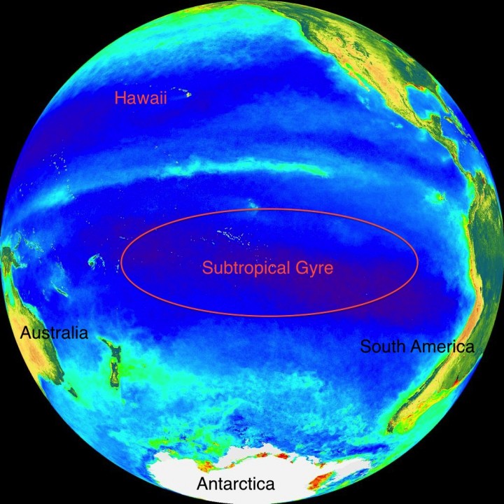
The P06 ship track, for the most part, follows along 32.5° of latitude south. That route places our course just south of the center of the South Pacific Gyre—the largest of the five major oceanic gyres, which form part the global system of ocean circulation. The Gyre—on average—holds the clearest, bluest ocean waters of any other ocean basin. This blueness is the macroscopic expression of its dearth of ocean life. We have seen nary a fish nor other ships since we departed Tahiti—this is not a major shipping route. Oceanic gyres are often called the deserts of the sea. On land, desert landscapes are limited in their capacity to support life by the availability of water. Here, lack of water is not the issue. Water, however, is at least the co-conspirator in keeping life from flourishing. Physics, as it turns out, is what holds the key to this barren waterscape.
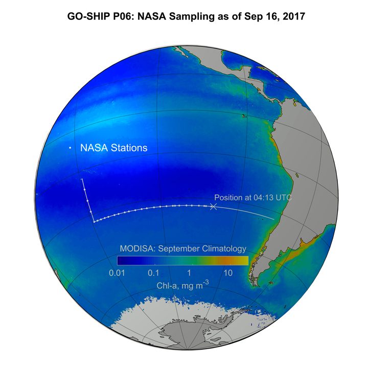
This map (above) shows the MODIS chlorophyll climatology with the ship track superimposed.
Due to the physics of fluids on a rotating sphere, such as our planet, the upper ocean currents slowly rotate counterclockwise around the edges of the center of the Gyre–as a proper Southern Hemisphere gyre should—and a fraction of that flow is deflected inward, towards its center. With water flowing towards the center from all directions, literally piling up and bulging the surface of the ocean–albeit, by just a few centimeters across thousands of miles–gravity pushes down on this pile of water. This relentless downward push puts a lock on life. The pioneers of life in the ocean, the tiny microscopic plants, known as phytoplankton, which drift in the currents, and grow on a steady mineral diet of carbon dioxide, nitrogen and phosphorus, and a dash of iron—and expel oxygen gas as a by-product, to the great benefit of life on Earth—must obtain most of their material sustenance from the ocean below. Layers of denser water trap the nitrogen and phosphorus-rich water at depth, keeping it too far down, where not enough light can reach it to spark the engine of photosynthesis that allows plants to grow.
Why are we here and where does NASA come into this story? Since the late 1970s, NASA has pursued—experimentally at first, and now as a sustained program—measuring the color of the oceans from Earth-orbiting satellites as a means to quantify the abundance of microscopic plant life. Microbiology from space, in a way. Formally, though, we call it “ocean color remote sensing.” Whizzing by at altitudes of several hundred miles, atop of the atmosphere, bound to polar orbits that allow satellites to scan the entire surface of the globe every couple of days, carrying instrument payloads of meticulously engineered spectro-radiometers—cameras capable of measuring the quantity and quality, or color, of the light that reaches its sensors. This is where our work aboard the R/V Palmer comes into the story. The data the satellites beam down from orbit do not directly measure how much plant life there is in the ocean. Satellite instruments give us digital signals that relate to the amount of light that reached their sensors. It is up to us to translate—to calibrate—those signals into meaningful, and accurate, measurements of plant life—or temperature, salinity, sediment load, sea level height, wind and sea surface roughness, or any other of the many environmental or geophysical variables satellite sensors can help us detect at the surface of the ocean. To properly calibrate a satellite sensor and validate its data products, we must obtain field measurements of the highest possible quality. That is what our team from NASA Goddard is here to do.
Around midday, typically the time of the ocean color satellite flying over our location, we perform our measurements and collect samples. We measure the optical properties of the water with our instruments to compare what we see from the R/V Palmer to what the satellites measure from their orbit above Earth’s atmosphere. At the same time that we perform our battery of optical measurements, we also collect phytoplankton samples to estimate their abundance, species composition as well as the concentration of chlorophyll-a, the green pigment common to most photosynthesizing organisms like plants, including phytoplankton. By collecting these two types of measurements at once, light and microscopic plant abundance, we are able to build the mathematical relationships that make the validation of the satellite data products possible.
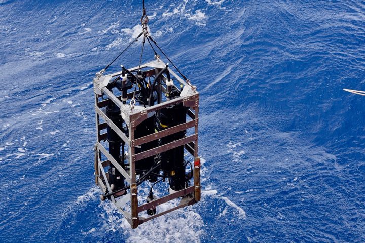
The optical instrument being lowered into the South Pacific Ocean. Credit: Lena Schulze/FSU
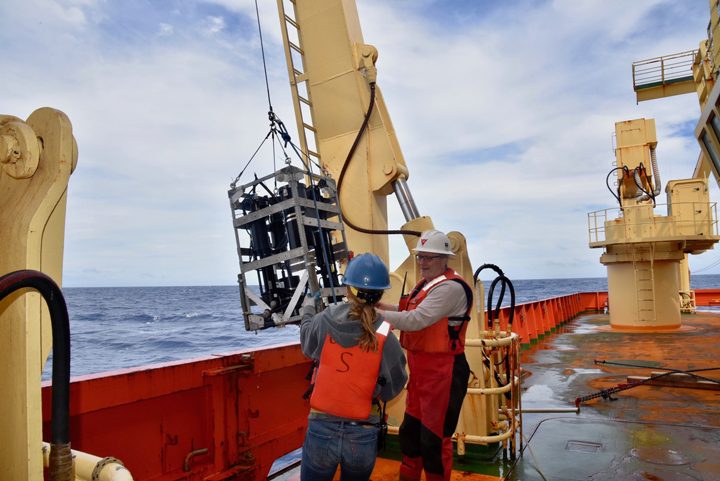
Scott Freeman of NASA works with a R/V Nathaniel Palmer crew member to prepare an instrument for deployment over the side of the ship to collect opHcal measurements. Credit: Lena Schulze/FSU
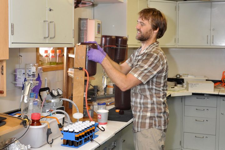
Mike Novack of NASA studies the optical and biological characteristics of seawater samples in the ship’s laboratory. Credit: Joaquin Chavez/NASA
The waters of the South Pacific Gyre are an ideal location for gathering validation quality data, perhaps one the most desirable to do so, because there are few complicating factors and sources of uncertainty that blur the connection we want to establish between the color of the water and phytoplankton life abundance. Our measurements will extend NASA’s ocean chlorophyll-a dataset to some of the lowest values on Earth. The water here is blue; in fact, it’s the bluest ocean water on Earth.
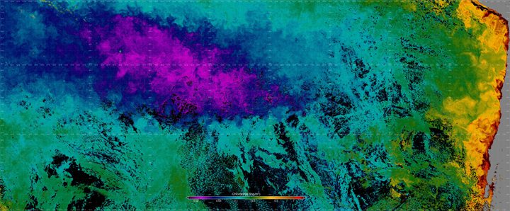
This false-color image is a composite, assembled from data acquired by the the Visible Infrared Imaging Radiometer Suite (VIIRS) on the Suomi NPP satellite between September 10-17, 2017. Yellow represents areas with the highest chlorophyll concentrations and purples are the lowest. Credit: Norman Kuring/NASA
My apologies for the gap between blog posts. My day job has been pretty busy. And even though the NASA folks have already arrived safely to Tahiti as of May 5, 2014, I thought it was fitting to have one last blog post. We have talked a lot about ocean biogeochemical sampling, ocean chemistry, and ocean color radiometry. It is also important to touch on the societal benefits that ocean color radiometry can provide.
In 2007, the International Ocean-Colour Coordinating Group or IOCCG published a report and an additional brochure entitled: “Why Ocean Colour? The Societal Benefits of Ocean-Colour Technology” and “Why Ocean Colour.” I will not go into all of the information detailed in each document here (though feel free to follow the links below at your leisure.)

IOCCG reports
A number of critical uses for ocean color are of particular importance in today’s society. For instance, detection of high algal biomass can indicate the location of potential fishing zone. Fish that eat algae or fish that eat fish that eat algae (did you get all of that?) will be en masse in these blooms. Inter-annual variation in timing and extent of phytoplankton blooms can also affect the survival of larval fish. Satellite imagery can be used to monitor this variation. Moreover, satellite derived sea surface temperature (SST) and wave height information can help aquaculture developers plan where to establish new fish farms. Satellite imagery can be used to detect and monitor blooms of harmful algae, algae (phytoplankton) that ether produce toxins or can clog the gills of fish and invertebrates because of high biomass.
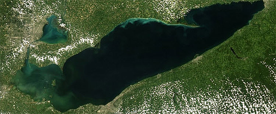
Harmful Algae Bloom in Lake Erie
http://oceanservice.noaa.gov/hazards/hab/
Satellite ocean color imagery is also very important for monitoring delicate ecosystems, particularly in global coastal environments. For example, the European Space Agency (ESA) has developed a program called CoastWatch that helps scientists harness the power of satellite imagery for monitoring water quality in shipping channels and coastal environments. The Medium Resolution Imaging Spectrometer (MERIS) on the Envisat platform (similar to NASA’s MODIS instruments) can be used to monitor sediment deposition onto coral reefs, which can smother the corals. The imagery can also be used to monitor water quality in shipping channels after dredging. Dredging can increase suspended sediments and negatively affect water quality.
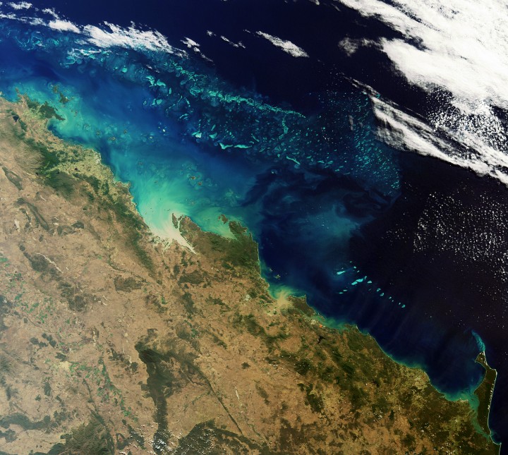
MERIS image: sediments flowing onto the Great Barrier reef in Australia
http://www.esa.int/Our_Activities/Observing_the_Earth/ESA_s_sharp_eyes_on_coastal_waters
Let’s consider a recent ecological disaster: the Deepwater Horizon oil spill. The Deepwater Horizon oil spill has been called the ‘worst oil spill in U.S. history’. The oil spill resulted from an oil platform explosion that occurred on April 20, 2010, and leaked an estimated 4.9 million barrels of oil by the time it was capped on July 15, 2010. This type of disaster can have long-term impacts on coastal wildlife and fisheries. Immediately following the spill, fishing areas around the Gulf Coast were closed to prevent human exposure to dangerous chemicals, polycyclic aromatic hydrocarbons, found in the oil. These chemicals are known to cause cancer. The fisheries were deemed safe and reopened on April 19, 2011.

Oil in the marshes of the Mississippi Delta
http://ocean.si.edu/gulf-oil-spill
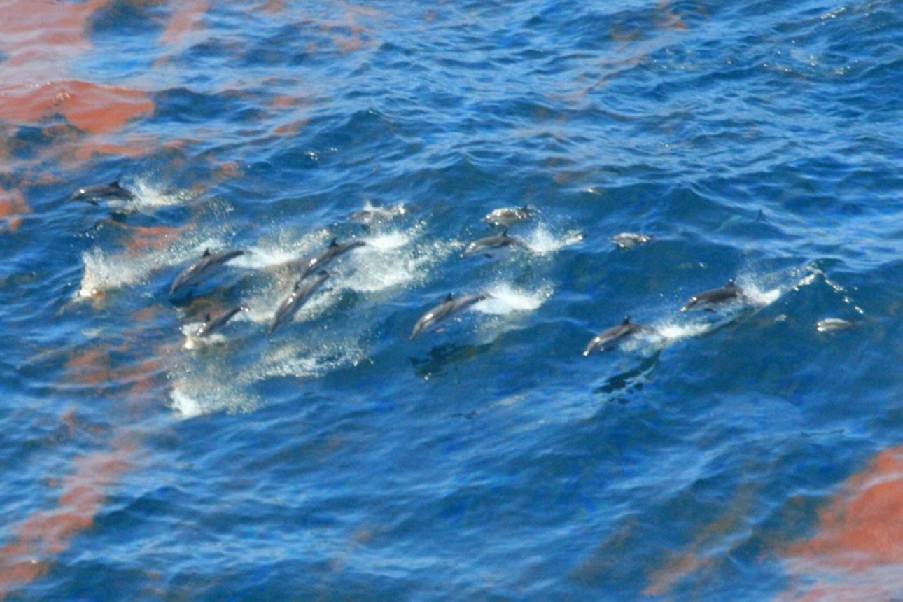
Dolphins swimming through the oil patches from the Deepwater Horizon spill
http://ocean.si.edu/gulf-oil-spill
Satellite ocean color imagery can be used to locate and monitor oil spills of this magnitude. Although this type of imagery is complex, the technology is a great asset. The video below, developed by video producers here at NASA Goddard, shows a timeline of NASA MODIS satellite images. Such imagery allowed scientists to follow the track of the oil slicks. These images can help us prepare for the impact of these disasters when we know where it is headed next. You can find satellite images of the oil spill here.
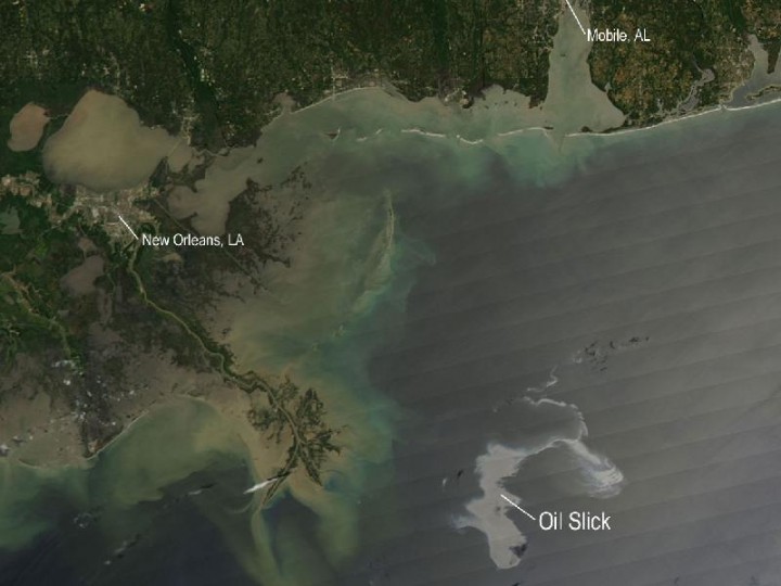
Satellite image of oil slick in the Gulf of Mexico following the sinking of the Deepwater Horizon platform
http://www.nasa.gov/multimedia/imagegallery/image_feature_1649.html
We have truly enjoyed sharing our experiences with all the blog readers. I hope we can do this again very soon. Until next time, make sure you check out all of the NASA field campaigns here at the Earth Observatory website.
http://www.ioccg.org/reports/report7.pdf
http://www.ioccg.org/reports/WOC_brochure.pdf
http://www.esa.int/Our_Activities/Observing_the_Earth/ESA_s_sharp_eyes_on_coastal_waters
http://www.esa.int/Our_Activities/Observing_the_Earth/New_ESA_project_supports_aquaculture
http://ocean.si.edu/gulf-oil-spill
http://www.nasa.gov/topics/earth/features/oil-spill-video.html
http://www.nasa.gov/topics/earth/features/oilspill/index.html
The global ocean is made up of five major ocean basins: the Pacific, Atlantic, Indian, Southern and Arctic Ocean. The Pacific Ocean is the largest of these basins as well as the deepest. Its expanse runs 155 million square miles and contains “more than half of the free water on earth.” Not only is it the largest and deepest ocean basin, but it is also the oldest, comprised of rocks that have been dated to be 200 million years old. You may have heard the term “Ring of Fire” associated with the Pacific Ocean. This name stems from the fact that the Pacific Ocean is prone to earthquakes and formation of submarine volcanoes along its extensive ridge and trench systems.
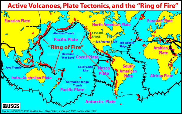
Ring of Fire
http://oceanexplorer.noaa.gov/explorations/05fire/background/volcanism/media/tectonics_world_map.html
The Pacific Ocean gained its name in the 16th century from the Portuguese navigator Ferdinand Magellan. Magellan and his crew set sail from Spain in 1519 in search of the Spice Islands located to the northeast of Indonesia. The Spice Islands were the largest producers in the world of spices such as nutmeg, cloves, and pepper. They navigated through the Atlantic Ocean and around the tip of South America after which they came across an unfamiliar ocean. He called this ocean ‘pacific’ which means peaceful. Unbeknownst to them, they still had a long journey to the Spice Islands. You can learn more about the voyage of Magellan and his crew here.
Magellan’s Voyage
http://news.bbc.co.uk/2/hi/science/nature/6170346.stm
OK, back to science! The CLIVAR P16S field campaign has entered the waters of the South Pacific known as a subtropical gyre. Gyre means “circular or spiral motion.” In the ocean, wind generated surface currents travel in a circular direction, either clockwise or counterclockwise, forming a large, circular body of water. The circular direction of the currents is caused by the Coriolis Force acting to deflect motion to the right in the Northern Hemisphere and to the left in the Southern Hemisphere due to the Earth’s rotation. The South Pacific gyre is located in the Southern Hemisphere, so winds and water are deflected to the left. Because of the deflection to the left, the gyre circulates in the counterclockwise direction, forcing water to pile up in the center of the gyre. In the last post, “An Appreciation for True-Color Satellite Imagery” we discussed how microscopic plants, or phytoplankton, require nutrients to grow. Blooms (large cell numbers) of phytoplankton cannot grow in these gyres because the water that piles up within the center of circulation is nutrient deficient.
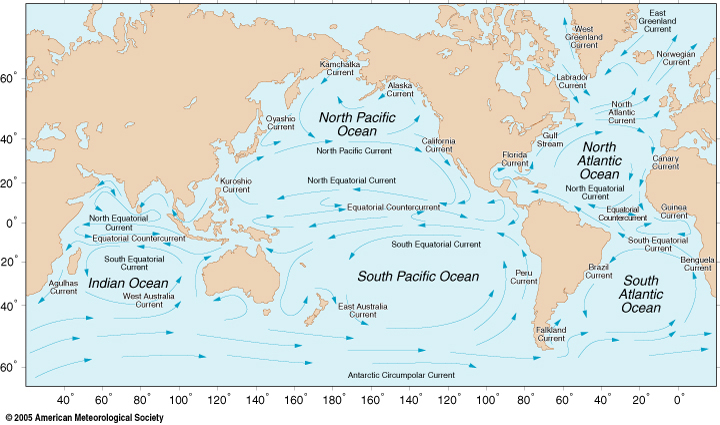
Global Ocean Circulation
http://oceanmotion.org/html/background/wind-driven-surface.htm
We can use the information about the color of the light being absorbed and reflected by the ocean to deduce the concentration of phytoplankton biomass using the proxy Chlorophyll a. Chlorophyll a is a pigment that both land plants and phytoplankton use to convert light to sugars in their chloroplast. Chlorophyll a absorbs strongly in the blue color of light. So when there is a lot of Chlorophyll a, then the light reflected back includes very little blue light. When there is very little or no Chlorophyll a, then a lot of blue light is reflected back. The figure below is an ocean color image based on the information I just described. The blue color represents little to no Chlorophyll a (or phytoplankton) present while the bright colors of yellow green and red represent increasing concentration of Chlorophyll a or phytoplankton biomass.
SeaWiFS Ocean Color image, Pacific Ocean
http://oceancolor.gsfc.nasa.gov/cgi/image_archive.cgi?c=CHLOROPHYLL
Please bear in mind that this explanation is very simplistic. You can learn more about how ocean color works here.
See the image below for the current cruise track of CLIVAR P16S. They are almost in Tahiti. Just a couple more weeks…
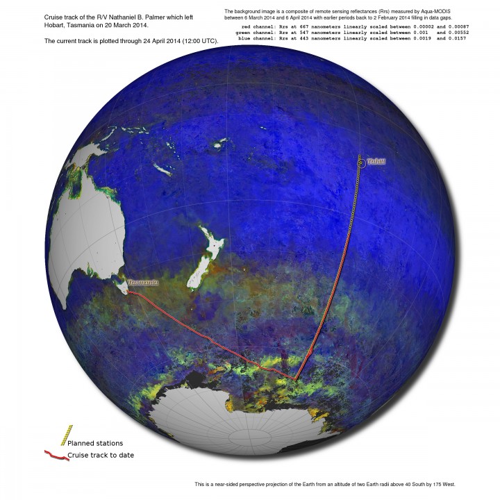
Cruise Track, CLIVAR-P16S
ACKNOWLEDGEMENTS: NASA’s Ocean Ecology Laboratory Field Support Group is participating in the US Repeat Hydrography, P16S field campaign under the auspices of the International Global Ocean Ship-Based Hydrographic Investigations Program (GO-SHIP). The US Climate Variability and Predictability Program (CLIVAR), NOAA and the NSF sponsor this campaign.

http://oceanservice.noaa.gov/facts/biggestocean.html
http://oceanservice.noaa.gov/facts/pacific.html
http://www.iol.ie/~spice/Indones.htm
http://www.rmg.co.uk/explore/sea-and-ships/facts/faqs/what-and-where-are-the-spice-islands
http://news.bbc.co.uk/2/hi/science/nature/6170346.stm
http://www.merriam-webster.com/dictionary/gyre
http://ww2010.atmos.uiuc.edu/(Gh)/guides/mtr/fw/crls.rxml
http://oceanworld.tamu.edu/students/currents/currents3.htm
http://oceancolor.gsfc.nasa.gov/cgi/image_archive.cgi?c=CHLOROPHYLL
http://oceancolor.gsfc.nasa.gov/SeaWiFS/
We have spent the last few weeks discussing the differences between inherent and apparent optical properties in the ocean and how we measure them. Now let’s take a moment to appreciate the information these data give us. I am sure many of you have seen satellite images of the ocean, hurricanes, etc. on the news and at other outlets. A lot of work goes into each and every one of those images and they can show remarkable things on a global scale that would be difficult to detect through fieldwork alone.
Below you will see a true color image of a phytoplankton bloom in the Barents Sea that was acquired on August 24, 2012 by NASA’s MODIS Aqua satellite . The Barents Sea is part of the Arctic Ocean and is located off the northern coasts of Norway and Russia. The word phytoplankton is Latin for plant (phyto) and to wander or drift (plankton). Phytoplankton can photosynthesize and produce energy from sunlight just like plants do on land. They also take up carbon dioxide and release oxygen like land plants. Phytoplankton are an important component of the food chain as other organisms such as zooplankton and fish use them as a food source. Additionally, they play an important role in the global carbon budget because they can use the carbon (CO2) that is absorbed by the ocean to make sugars.
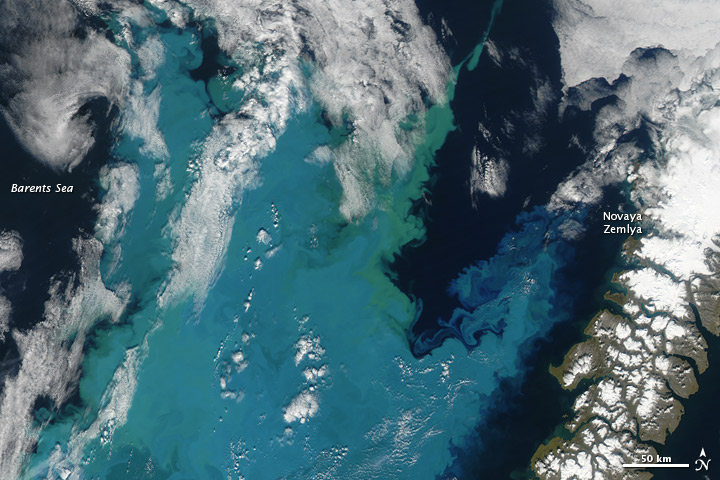
Barents Sea phytoplankton Bloom
There are many types of phytoplankton that bloom in the ocean including diatoms, dinoflagellates, and coccolithophores, just to name a few. You can learn more about different phytoplankton groups here. They all rely on specific nutrients, such as nitrogen (NO3, NO2, etc.), phosphorous (PO4, etc.) and trace metals (iron, magnesium, etc.). Phytoplankton blooms occur when many individuals, or cells, of one species are present in one region of a body of water (lake, estuary, open ocean), altering the color of the water. In the image above, the water is dominated by a species of coccolithophore. Coccolithophores are a type of phytoplankton that are covered with plates made of calcite called coccoliths. Calcite, or calcium carbonate, is white giving that creamy white look to the water. You can learn more about this coccolithophore bloom here.
This next image was recently featured on NASA’s OceanColor website. It was taken off the western coast of Africa where a current called the Benguela current flows northward bringing water from the South Atlantic and Indian Ocean. In this image from April 10, 2014 we can see a yellow discoloration in the water. I just learned that this area is prone to toxic hydrogen sulfide precipitation events that have been known to cause fish and other marine animal mortalities. Amazingly, these events have been captured using satellite imagery. However, the cause of this particular discoloration has not, as of this post, been determined. This is where fieldwork comes in! Still, it is very cool! Thanks to Norman Kuring at NASA Goddard for locating this feature.

Discoloration in the Benguela Current off the coast of Namibia
You can enjoy many other satellite images at NASA’s Visible Earth website.
References:
http://www.worldatlas.com/aatlas/infopage/barentssea.htm
http://earthobservatory.nasa.gov/Features/Phytoplankton/
http://www.bigelow.org/foodweb/microbe0.html
http://protozoa.uga.edu/portal/coccolithophores.html
http://oceancolor.gsfc.nasa.gov/
http://oceancurrents.rsmas.miami.edu/atlantic/benguela.html
http://oceancolor.gsfc.nasa.gov/cgi/image_archive.cgi?i=423
http://www.sciencedirect.com/science/article/pii/S0967063703001754
ACKNOWLEDGEMENTS: NASA’s Ocean Ecology Laboratory Field Support Group is participating in the US Repeat Hydrography, P16S field campaign under the auspices of the International Global Ocean Ship-Based Hydrographic Investigations Program (GO-SHIP). The US Climate Variability and Predictability Program (CLIVAR), NOAA and the NSF sponsor this campaign.

One of the greatest tools used by oceanographers today for measuring ocean processes is the CTD. CTD stands for Conductivity, Temperature and Depth. Conductivity is a measure of ocean salinity. The CTD is used to collect profile data in the ocean. The CTD is typically accompanied by a carousel, or rosette, of large bottles (Niskins) that can hold about 10 liters (2.6 U.S. gallons) of water. Some Niskins are large enough to hold 30 liters. These bottles have spring-loaded caps that can be triggered to close at specified depths. The CTD and other sensors, such as a chlorophyll fluorometer, and an Acoustic Doppler Current Profiler (ADCP) that measures current velocities, and other sensors can also be attached within the rosette package.
The whole package is connected to a very long cable and is mechanically lowered by a winch operator down through the water column, which is called the ‘downcast.’ During the downcast, information about salinity, temperature, depth and data from the other sensors are sent to a computer on board the ship. The computer is connected through the cable that is lowering the package. The downcast is halted once the package reaches close to the ocean floor. When the CTD is raised back to the surface, the ‘upcast’, each of the Niskin bottles is closed at assigned depths, collecting water as it travels back to the surface.
Once the Rosette package is back aboard the ship, the scientists are able to collect water from the bottles for their analyses. The parameters collected and analyzed during CLIVAR campaigns includes but are not limited to: salinity, oxygen, nutrients, chlorofluorocarbons (CFCs), dissolved inorganic carbon (DIC), total alkalinity, pH, dissolved organic carbon (DOC), helium, and tritium.
Certain compounds, such as some radionuclide (tritium, carbon-14, etc.) and CFCs, can be used as ‘tracers’. These tracers are used to follow ocean currents and calculate the age of water parcels. CFCs were prominently used in refrigerators and air conditioning units until the 1970s when they were banned over the concern of ozone depletion. You can learn more about the CFC tracer program here. Through the WOCE and CLIVAR programs CFC concentrations have been measured all over the world.
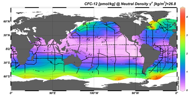
Map of global CFC measurements
http://www.pmel.noaa.gov/cfc/
The measurement of pH, total alkalinity and DIC are important for monitoring ocean acidification. Ocean acidification (OA) is the decrease in ocean pH as a result of an increase in carbon dioxide (CO2) absorption by seawater. OA is a prominent concern in today’s world. CO2 is pumped into the atmosphere from everyday human activities, such as emissions from vehicles and industrial pollution. Each year approximately 25% of the CO2 pumped into the atmosphere is absorbed by the ocean. Although plants can use CO2 for photosynthesis, the increase also has negative implications. As the amount of CO2 absorbed by the increases, the pH is expected to continue decreasing.
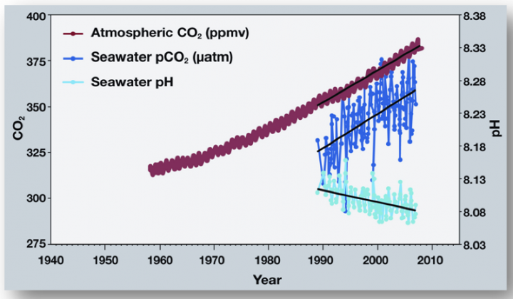
pH time series
http://www.pmel.noaa.gov/co2/story/OA+Observations+and+Data
The pH of the ocean directly affects organisms that form calcium carbonate shells or structures, like corals, oysters, clams and sea urchins. An acidic environment causes the calcium carbonate to dissolve and makes it more difficult for the organisms to make their calcium carbonate skeletons. Therefore, it is important that programs like CLIVAR are monitoring global CO2 concentrations (part of the DIC pool), total alkalinity (the ability for the ocean to neutralize acids) and pH. We know that decreases in ocean pH can negatively impact marine organisms. You can see more about the effect of ocean acidification or marine organisms here.
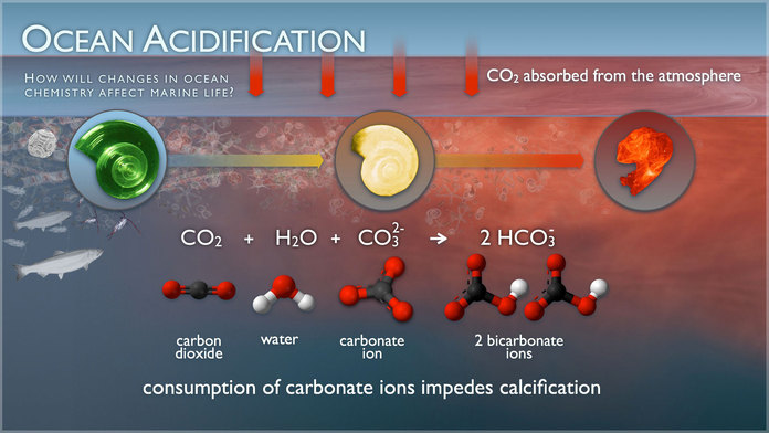
Ocean Acidification
http://www.pmel.noaa.gov/co2/story/What+is+Ocean+Acidification%3F
As I was conducting some research for this blog post I came across this article that was posted at the Earth Observatory in 2008 about the global carbon budget. I thought it was appropriate to bring it back here.
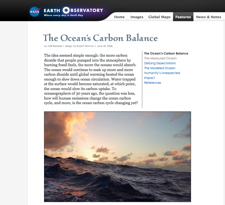
Earth Observatory article from 2008
References:
http://www.whoi.edu/home/oceanus_images/ries/calcification.html
http://www.pmel.noaa.gov/co2/story/What+is+Ocean+Acidification%3F
http://water.me.vccs.edu/exam_prep/alkalinity.html
http://earthobservatory.nasa.gov/Features/OceanCarbon/
http://rspb.royalsocietypublishing.org/content/275/1644/1767.full
ACKNOWLEDGEMENTS: NASA’s Ocean Ecology Laboratory Field Support Group is participating in the US Repeat Hydrography, P16S field campaign under the auspices of the International Global Ocean Ship-Based Hydrographic Investigations Program (GO-SHIP). The US Climate Variability and Predictability Program (CLIVAR), NOAA and the NSF sponsor this campaign.
