By Lora Koenig
Byrd Station (Antarctica), 9 December — Today was a huge day. First off we figured out the problem with the radars: One of the USB ports on the computer was not functioning properly. When we changed the USB port, the problem went away. I was relieved there was such a simple solution to the problem and so was Clem, who had had a rough night’s sleep worrying about the radars.
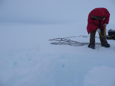
At around 9 AM we headed out to drill our first ice core of the season. We drilled at a site about 3 kilometers (1.86 miles) away from camp. This site was chosen because a previous ITASE core was drilled there in 2002. Our core will update this core and we will compare the overlapping years of ours with ITASE’s to understand any differences. Last year we also drilled at a site of a previous ITASE ice core and got similar results that give confidence in the measurements and methods from both cores.
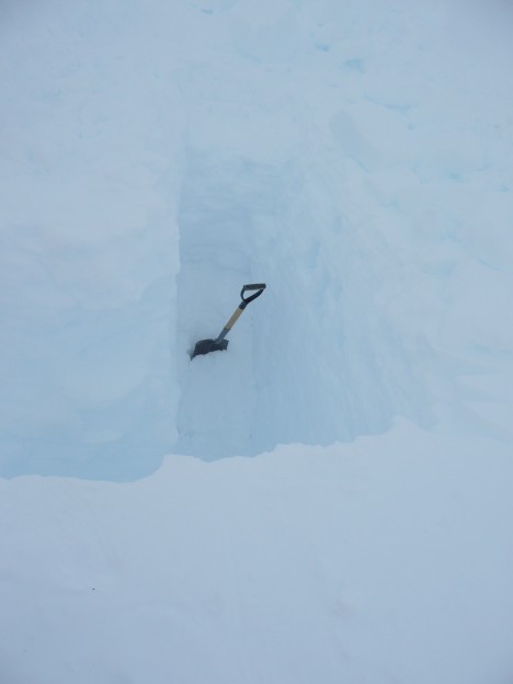
Clem ran the radar out to the drill site to image the layering while Ludo drove the snowmobile. Once at the site, Ludo immediately started digging the snow pit to sample the snow in the top 2 meters (6.56 feet) of the ice sheet. The snow at the very surface of the ice sheet is very similar to the hard wind-packed snow that you would encounter in the high mountains in the U.S. and it’s not bonded well enough for us to ship cores of it back to the U.S. in one piece, so instead we took samples of the snow in the pit for lab analysis. The cores have to stay in one piece, or we would lose our chronological record. Additionally, we took other measurements in the snow pit that are important for modeling how the microwave radiation, from both the satellites in space and radars on the ground, interacts. Snow grains of different sizes and shape can actually be detected by satellites in space! As the snow grain size changes, the signals in space change.
Ludo spent all day in the pit. We think he may hold the record for the most time in one pit, about nine hours from digging to fill in. He took infrared photographs of the snow. Here is one from the pit:
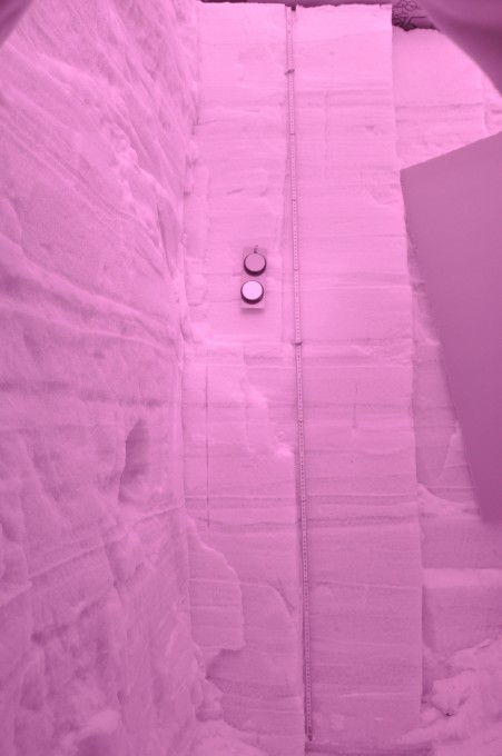
These photographs are used to calculate the grain size given the different reflectance levels of the infrared radiation. The photos are pink because they are taken in the infrared wavelength, not visible light like most cameras do. They are also very pretty to look at and you can see all of the layers of snow. Each storm puts down a new layer of snow. There was a new layer approximately every 6 cm (2.36 in) in this pit. There were more layers than I have ever seen before in a pit, which made the pit measurements take such a long time.
At about a third of the way down the picture the snow becomes firn, which is snow that had persisted through at least one melt season. We cannot tell from the snow pit exactly how old the firn in the pit is (we need the isotopes for that), but we know that there are at least three years of records in the pit, so the firn at the bottom could be from 2009.
After the infrared photos, Ludo recorded the stratigraphy of the pit (snow grain size and type) using a macroscope, cut snow samples for isotopic analysis, and measured the thermal conductivity of the snow, which is the snow’s ability to transfer heat. Heat conducts through the ice lattice more than through the air in the pore spaces, so thermal conductivity is also a measure of how bonded the snow is. Because I was helping Ludo in the pit there are not any photos of this process. Often while we are actually doing the science we don’t have many photos because we are all working.
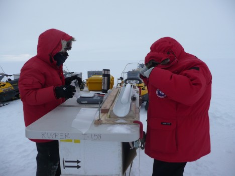
As Ludo was working in the snow pit, Randy started drilling the ice core. He would drill the core and Jessica and Michelle would process it. The core is weighed and measured to calculate its density. The length of the core and the depth of the drill hole are recorded, and the electrical conductivity of the core is measured to detect changes in snow chemistry. The core is then put in a bag, a tube and a box for shipping back to the lab for isotopic analysis. The final depth of the core was 16.8 m (55.1 ft), which will correspond to about 40 years of snow accumulation history.
By Lora Koenig
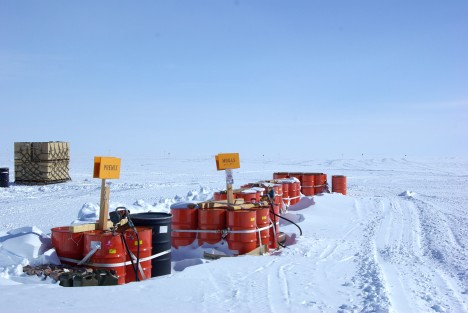
Byrd Station (Antarctica), 8 December — Today was our first day in the deep field at Byrd Camp. Byrd Camp sits in the middle of the West Antarctic Ice Sheet at an elevation of about 5,700 ft (1,737 m). We are standing on over 2,000 m of ice, with the oldest ice being about 50,000 years old. (The ice nearby at WAIS divide camp is a bit older and deeper. To find out more about the deep ice underneath us check out this information on the WAIS Divide ice core, which is being drilled deep into the ice nearby.) When you look out from camp you see nothing but the flat white snow and an old drill tower sticking out of the ground.
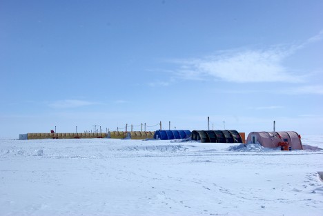
We are, specifically speaking, at Byrd Surface Camp. The original Byrd Camp, established in the 1956-1957 season, is underneath us, except for a drill tower that still sticks out above the snow. Over the years, snow accumulation (which averages around 12 cm per year at Byrd) buried the original camp and created Byrd Surface Camp, which everyone just calls Byrd. It is exactly this snow accumulation that we are here to measure with ice cores and radars. Here is an article about the history of Byrd.
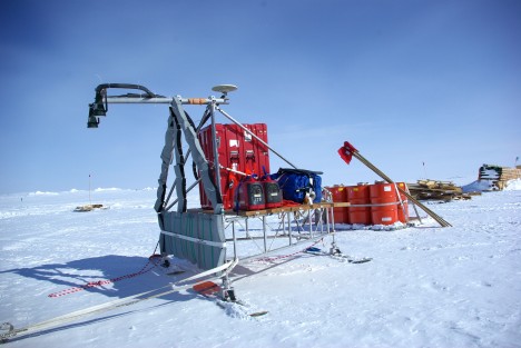
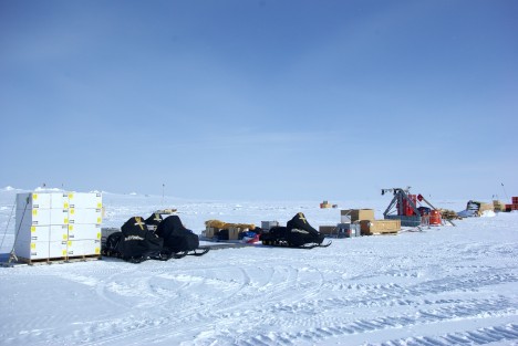
The team was prepared to work hard today because we know the more time we make up from the weather delays, the quicker the traverse team can get home. The day started with all of us breaking down the pallets of gear. Once all the gear was off of the pallets, we divided and conquered the tasks for the day. Michelle started loading and organizing the sleds. Randy fueled all the snowmobiles and Jerry cans. We brought nine 55-gallon drums of premix gas for the snowmobiles for the entire traverse. Jessica prepared all of the drilling gear for the first core, which we’ll drill tomorrow. Clem, Ludo and I built the radar sled, attached the antennas and hooked up all of the radars for testing. Clem also set up a GPS base station that we will use to correct our roving GPS on the radar so we know precisely where the radar data is located throughout the traverse.
We discovered a few problems today. First, Jessica realized that the power converter for the drill battery did not make it to the field. The drill is made in Switzerland and has a different power plug. While this was an unfortunate oversight, it will not affect the science: We can charge the drill battery with the solar panels. The sun is up 24 hours a day here, so that will provide more than enough charge for the battery. Also, we carry an electronics tool kit, so in case of need we can cut the wires and make a new plug.— we call it “MacGyvering” (i.e., improvising fixes to our materials in the field).
The second problem of the day is a bit more worrisome. The Ku-band radar data has a systematic noise level that we cannot troubleshoot. We know that it has something to do with the computer that runs the radars, but we cannot determine whether or not the problem is coming from radio frequency emission from the computer itself getting into the antennas or if it is a data writing problem with the computer software. It has been a long day, so the trouble-shooting will have to be left for tomorrow. We hope that nothing was broken on the computer during the combat off-loading. We will know more tomorrow.
The sleds are ready to drill our first core tomorrow!
By Lora Koenig
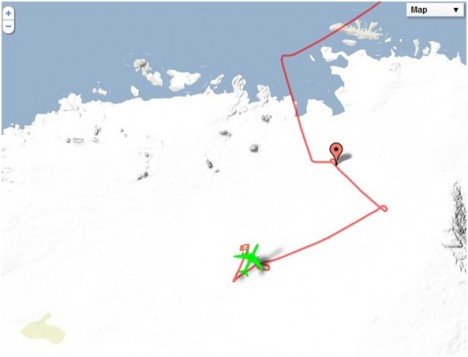
Yesterday was an exciting day in the office. While I was downloading satellite data, answering e-mails and tying up loose ends before leaving for Antarctica, I was also closely following the NASA Airborne Sciences Flight Tracker and the flight path of the NASA DC-8 aircraft. The DC-8 is currently flying over Antarctica as part of the Operation IceBridge mission and yesterday it overflew the 2010 SEAT traverse line and ice core drilling sites. (For more detailed info on Operation IceBridge, check out the mission’s website).
I spent part of the day yesterday watching my screen as the flight tracker showed a little green aircraft moving over our 2010 route. Here is the aircraft approaching our line at about 1:40 PM Eastern time. (The tracker was not updating the plane image at this time, but the aircraft was at the end of the red line.)
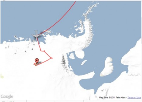
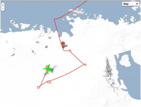
Here it is halfway through. (Note that the plane does a 270-degree turn to line up on our traverse line to make sure it is leveled as it crosses our 2010 ice core sites. This ensures the best quality of radar data.)
And here is the plane at about 2:35 PM EST, finishing the portion of its flight that retraced our traverse and four ice core locations:
I watched on my screen as the IceBridge plane covered in just less than an hour the same ground that took us 12 days to cover last year.
OK, so I guess you are asking yourself: Why do we go out in the field, in sub-freezing weather, to drive around on snowmobiles for 12 days to do what a plane can do in an hour? Because you can not drill an ice core from an airplane. The airplane carries radars, which provide great spatial coverage of radar data, but we need to calibrate the radar data with the annual cycles we get from ice cores. (See last week’s blog post on how we determine annual cycles in the lab). So, yesterday, IceBridge collected great radar data that will compare to the data from our ice core sites, as well as to data from the WAIS divide ice core and the ice cores collected by a group led by Dr. Ian Joughin at University of Washington.
The IceBridge DC-8 aircraft flies with radars that are nearly identical to the ones we use on the ground. They are named Snow Radar and Ku-band Radar and are built by the Center for Remote Sensing of Ice Sheets, CReSIS. We will use the airborne radar data gathered yesterday to investigate any differences between what the radars are measuring from the air and on the ground.
In a week, we board our flights to Antarctica. After watching the IceBridge plane flying in West Antarctica yesterday, I am even more excited to get my boots on the ice.
By Lora Koenig
Two weeks ago, I traveled to Utah to help the team finalize planning for this season and to visit the ice core lab and our 2010 ice cores at BYU. The entire was there, except for Ludo, who was in Hawaii competing in a triathlon. (Ludo is not only a top scientist but a top triathlete. I hope he is not getting too use to the warm weather because in less than a month he will be facing temperatures around 0°F.)
There were a few tasks to complete in Utah. The first was to look at many different types of satellite data on the region where we will be traveling to make sure there aren’t any crevasses or other dangers along the route. A crevasse is a crack in the ice. As the ice flows (yes, ice flows just like a mound of putty), it can crack when it goes over a bump or accelerates. Here is a recent picture of crevasses in Western Antarctica, from a NASA Operation IceBridge flight.
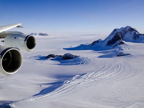
As you can imagine, we would not want to drive a snowmobile in an area like this. So we spent hours looking over maps of the rock bed under the ice sheet to look for bumps, visible and radar satellite images of the surface of the ice sheet, and satellite data showing the velocity of ice flow to make sure that we are traveling on the safest possible route. We ended up moving one ice core drilling location slightly to avoid a dark spot that we could not clearly identify in one of the radar images, just to be extra cautious. Once the route was established, we generated waypoints (coordinates) every kilometer to load into the GPS units that we will use for navigation. The place we are going to is big, white and flat: It is very easy to lose your sense of direction, so we rely heavily on GPS units for navigation.
For some great images and videos on how ice flows in Antarctica please check out this video, made by our NASA colleague Eric Rignot who (thanks again, Eric!) also checked the data that sits behind these videos to help ensure our safe route.
If you would like an in-depth look, this file, which opens on Google Earth, shows our final route with points every 1 km.
Our second task in Utah was to visit last year’s ice cores and have our first meeting to discuss the initial data coming from them. First, here is a picture of a core in the field, taken in December 2010.
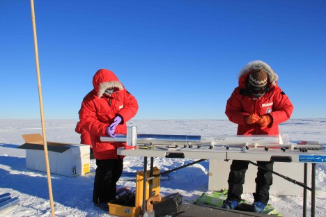
In this photo, Michelle (right) is labeling the core and I (left) am getting the core tube ready for storage. The arrow on the ice core bag shows which direction is up. It is very important that all the cores are labeled in order, or we would lose our time series. The metallic tube in the center left of the picture protects the core during shipping. The core in the tube gets placed in the white core box sitting open on the left side of the picture. (Also, notice that Michelle is standing on a bright green pad to help insulate her feet from the cold snow. It’s a veteran trick for keeping your toes warm.)
Here is that same core in the lab today.
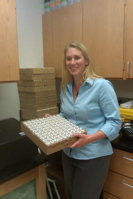
Summer is holding what was about 8 feet of the core and the rest of the about 50 feet of core is stacked in the boxes behind her, waiting for analysis.
Here is a very basic explanation of what happens to the cores once they arrive at Summer’s lab at BYU. (Normally, Summer would be the one writing this, but she is currently studying glaciers in Bhutan.)
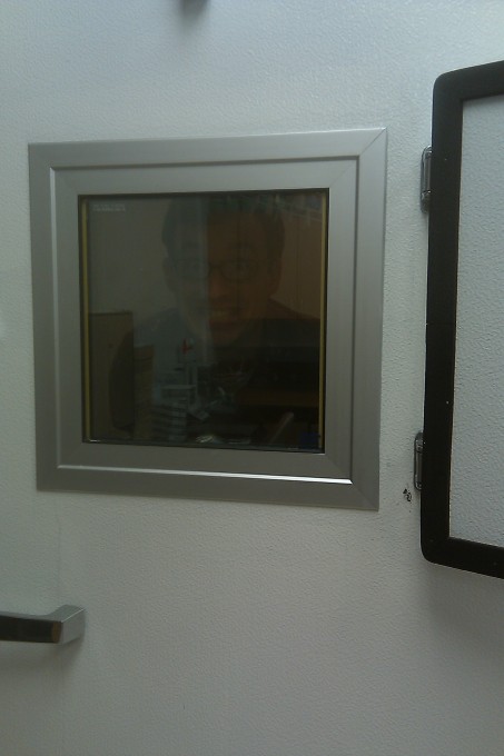
When the core arrives, we put it in the freezer. Here is Landon peering out of the freezer door:
In the freezer, we weigh the core to determine its density and measure its electrical conductivity, which tells us about its chemical composition. A volcanic event would be detected in the cores by the electrical conductivity and can be used to set a point in time. We take all these measurements twice, or even three times, to make sure they are accurate.
Here is a picture of a core that Landon is preparing, sitting on the freezer’s core handling tray:
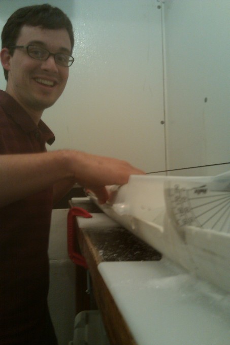
This freezer is set to -4°F, so when not posing for a picture, Landon would normally be in a parka with gloves on. As you can see, the core is still in its protective bag, which will be removed when actually processing the core. From here, the core is cut up into sections less than an inch (2 cm) long, and melted for the next stage of analysis.
I will add a quick note here that on last year’s traverse Landon was our lead driller. Both Landon and Jessica are masters students at BYU. They are not only integral players of the field teams, but are also the lead students for the lab analysis of these cores.
Once we have melted the core and put it in a bottle, we send it over to Jessica.
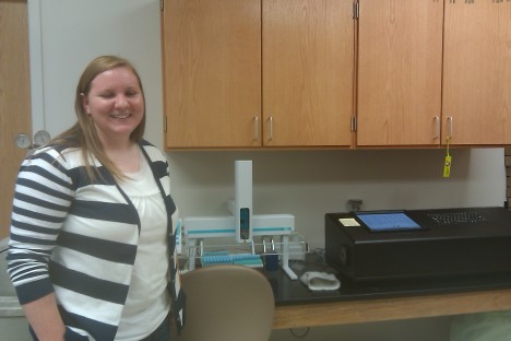
Here is Jessica operating the mass spectrometer (black box to the left in the picture with the blue screen) that will measure the stable water isotopes used to date the core. The isotopes in the snow have an annual cycle and it is this cycle that determines age of the core. An isotope is an atom, in our case an oxygen atom, that has different variations with different number of neutrons and atomic numbers. Oxygen has three stable isotopes: 16O, 17O, and 18O. The peaks and valleys in the ratios of 18O/16O reflect the warmer (summer) and cooler (winter) temperatures, respectively. Once the mass spectrometer determines the number of isotopes, we can establish the age of the core, in a way similar to counting tree rings. During this process, the core is in the little blue vials just to the right of Jessica.
After spending some time in the lab, we looked at the data from the first core that has been analyzed. At this point the density and isotopes have been measured and Summer is carefully working to put together the depth-age scale, which is the age of the core at each depth where the core use to sit in the ice sheet. I will use the density data from the core to determine an age-depth scale from the layers in the radar data and if all goes well the radar and ice core will line up giving us confidence in our analysis.
Last Monday, when I returned to Goddard, I had received my travel itinerary. We will be leaving the U.S. on Nov 17th to make our journey down to Antarctica. With all of this preparation, I am eagerly awaiting getting my feet on the Ice.
