By Eric Lindstrom
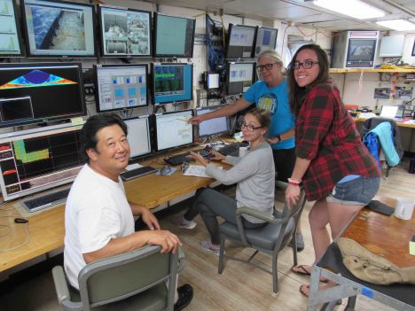
The CTD team (Spencer, Leah, Janet, and Kristin).
The focus of SPURS-2 is the upper ocean and the fate of rainwater. However, in order to study the top of the ocean one needs to know what is going on deeper down. The beauty of SPURS-2 is not skin-deep! SPURS-2, like many prior physical oceanography experiments, requires a basic background and context of the ocean circulation environment upon which many of our other more specialized or detailed measurements can be interpreted. The two major pieces of the contextual information for us are the surface circulation and the surface salinity pattern.
The surface salinity pattern is provided by remote sensing for the largest scale and by the array of drifters and profiling floats that have been deployed with salinity sensors. Also, the R/V Revelle is collecting a treasure trove of upper ocean salinity measurements wherever she goes – with continuous underway measurements of salinity from intakes at the surface, 2 meters (6.5 feet), 3 meters (9.8 feet), and 5 meters (16.4 feet) depths. I’ll go into that in more detail in a later blog on the Surface Salinity Profiler.
The surface circulation of the ocean is largely the result of the wind and the shape of the massive deep layers below the surface. In fact it can be crudely estimated if one knows the precise shape of the thermocline – the boundary between the warm upper ocean and the vast deep cold ocean. Here in the tropics the thermocline is pretty well represented by the 20°C (68° F) isotherm. Think of the warm upper ocean as all the water warmer than 20°C and the layer below as all the water colder than 20°C. Tropical oceanographers can use the depth of the 20°C isotherm much like meteorologists use surface atmospheric pressure maps to chart the highs and lows of weather and their associated winds. Here, if the 20°C isotherm rises toward the surface locally it is associated with a counterclockwise ocean surface current. The signature of the westward North Equatorial Current is a gentle slope of the isotherm from deeper in the north to shallower in the south. This is where our Conductivity-Temperature-Depth (CTD) instrument comes into the SPURS-2 plan. We can use it to track the shape of the thermocline. I wrote about the CTD during the SPURS-1 campaign. It is still the workhorse of physical oceanography – or maybe the monkey on the back of every physical oceanographer! Our show seldom goes on without it.
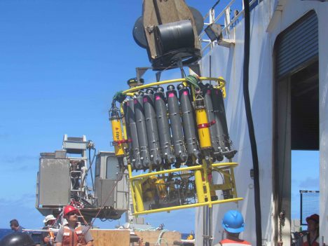
Preparing the CTD to go over the side.
Janet Sprintall from Scripps Institution of Oceanography and her team (Spencer Kawamoto, Leah Trafford, and Kristin Fitzmorris) are now mapping the temperature and salinity structure of the ocean well into the deep cold abyss (to 1.5 kilometers –0.93 miles– below the surface). The ocean depth is about 4.5 kilometers (2.8 miles) and the lower 3 kilometers (1.86 miles) are (for our purposes) relatively uniform and cold. Janet has planned a grid of 49 stations 30 miles apart around the SPURS-2 central mooring. These will be completed over about a week’s time. Simultaneously there will be regular sampling with the Surface Salinity Profiler between some of the CTD stations and we will optimize our meteorological measurements by limiting our speed to 10 knots (11.5 mph). So, while studies of the meteorology and near surface salinity are ongoing, as we move about the ocean, Revelle stops for an hour every 30 miles to collect necessary information on the background oceanographic conditions.
The CTD instrumentation remains largely unchanged (although perfected) in recent decades. Temperature, salinity, and oxygen sensors are mounted on the bottom of a large frame. Water sample bottles are mounted around the outside of the frame. Other instruments, such at the acoustic Doppler current profiler, may also be mounted on the frame. All data is transmitted up the conducting wire cable that is used to raise and lower the instrument. This bulky package is now easier to deploy and recover than in yesteryear due to innovations on today’s vessels. Now the Revelle has a specialized mechanical arm to get the CTD over the side and back on deck safely without much human intervention.
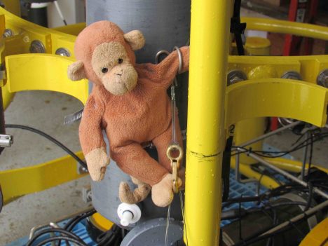
Monkey climbing over the water sample bottles on the CTD.
For my entire career oceanography has been spelled “CTD.” Knowing the temperature and salinity structure from surface to ocean depths is the key to our understanding of the ocean’s role in climate. The first global mapping of these characteristics (with CTDs) was not realized until the World Ocean Circulation Experiment in the 1990’s. Now oceanographers are working hard to understand all the physical, chemical, and biological changes associated with global warming, rising carbon dioxide levels, and industrial fishing. In that big picture, SPURS-2 might look like a small bit of monkey business over the tropical thermocline. However, we know that the resulting scientific understanding will long outlive the memory of our tiny field program in this vast Pacific Ocean!
ATom-1, the first of four ATom deployments over the next few years, is about to wind down. We’ve covered over 60,000 km and flown all the way around the world, but unlike the Jules Verne classic, it took us only 24 days (and not 80) to make it back to Palmdale, California. I managed not to get sick (or break any bones, which is an achievement if you know me!), despite the nearly 100 flight hours and lots of sleep deprivation.
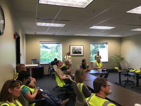
Tired ATom scientists at our final pre-flight briefing. Photo by Róisín Commane
I have found the second half of the ATom-1 deployment a lot more challenging than the first half. Some of the challenge was the constant changing of location and lack of routine outside of the aircraft. It has gotten to the stage that I might not know what city I’m in, what day it is or what the local time is, but I can get the instrument ready to measure. That’s both comforting and a little disturbing!
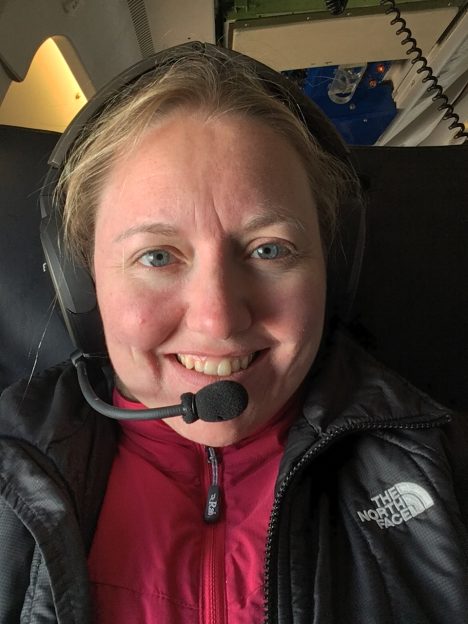
Róisín Commane trying to stay warm on the final ATom flight. Photo by Róisín Commane
Some of the challenge was the fatigue brought on by the long length of working days on the aircraft and time changes, the effects of which I didn’t fully appreciate beforehand. On a typical flight day we wake up at 3 a.m. to shower and pack our bags, we start preparing the instrument for the flight at 4 a.m., we take off at 7 a.m., fly and measure for 10 hours, and land at 5 p.m. if we don’t change time zones. As we constantly fly to a new location, it then takes another hour or two to get off the aircraft and to the hotel. With such a long flight day, all I’m able to do after a flight is fall into bed – ideally after finding some food!
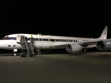
Preparing to leave Punta Arenas, Chile in the dark. Photo by Róisín Commane
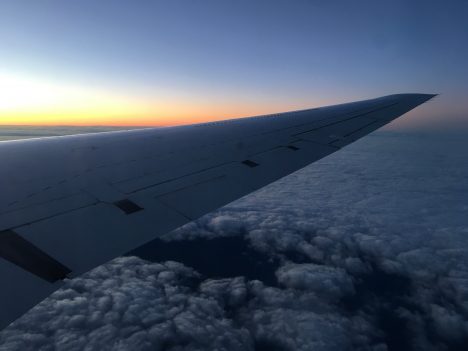
Flying into the sunrise. Photo by Róisín Commane
Flying east was a lot harder than flying west and to help this I think we are planning an extra day in Punta Arenas, Chile for ATom-2. We needed more than a day to get back on track after an 8 hour time change. It was winter in Punta Arenas this time so it was a little too cold to spend long in the sunshine (to encourage my sleep cycle to normalize). But in February, it will be southern hemisphere summer and being outside will be much easier. And hopefully I will fulfill a long-time ambition and see a penguin in the wild next time too! And not just a black and white cormorant that looks like a penguin!
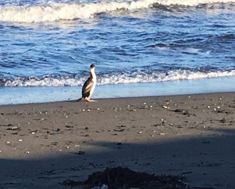
A cormorant on the beach in Punta Arenas, Chile. Hopefully next time I’ll see a penguin! Photo by Róisín Commane
By Eric Lindstrom
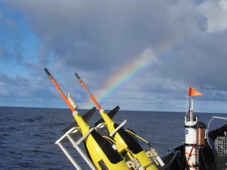
Instruments ready for Lagrangian array deployment at the end of the rainbow.
What do Leonhard Euler (1707-1783) and Joseph-Louis Lagrange (1736-1813) have to do with SPURS-2? How do we have two experiments going on simultaneously honoring the work of these famous mathematicians?
Two frames of reference have taken their names from these 18th century mathematicians. In science, including oceanography, when we make measurements of fluid flows fixed in space, we watch properties such as temperature or salinity as currents carry them by our instruments. This is called an Eulerian frame of reference. However, sometimes we make measurements while following the flow, trying to tag a parcel of water and watch as it moves and changes over time. This water following perspective is called the Lagrangian frame of reference. For example if you watch a river flow past from the bank, you are using an Eulerian frame of reference. If you examine the river from a boat flowing with river, you would be making a Lagrangian observation of the river.
In SPURS-2 we use moorings and a fixed grid of stations to describe a patch of ocean as the water passes by. Moorings, stations, and satellites provide the Eulerian perspective over the year of SPURS-2. We use a variety of drifters, autonomous vehicles, and profilers (instruments embedded in the moving water parcels) to also build an extensive Lagrangian view of the ocean over the year. We use the Lady Amber over the course of the year to service and reset some of the Lagrangian experiment as those assets drift away from the study site. We use the Revelle to deploy the Eulerian array and to seed the ocean with the Lagrangian instruments to be tended at later times by Lady Amber. It really is two experiments united to understand the salinity patterns and movement of freshwater in the ocean!
Audrey Hasson driving the A-frame during mooring deployment.
During the Revelle voyage we are also planning a short-term (48-72 hour) Lagrangian experiment capture the processes by which rainwater mixes into the ocean. We will launch drifters specially designed to follow the surface current during a rain event and then follow them for day or two. We will sample the region around the drifters using the Revelle to further examine the changing temperature and salinity properties of the upper ocean. The Revelle will attempt to take several snapshots of the ocean conditions as the Lagrangian array disperses over a day.
Together our Lagrangian and Eulerian sensor arrays constitute a sensor web in the ocean. This sensor web captures ocean motion and salinity changes (particularly) on a wide range of time and space scales. This allows us to analyze processes that lead to changing surface salinity all the way from minutes to seasons and from millimeter size turbulence to major ocean currents. We cannot measure all things we would like all the time and in every place, so we have tuned our effort and sensor web design to provide enough information to estimate what we would like to know. We would like to know about the role of turbulent mixing at the surface; we would like to know the role of eddies in transport of freshwater; and we would like to know how the major equatorial currents impact the eastern tropical Pacific low salinity pool. Obtaining such knowledge of the ocean is ambitious and challenging. SPURS-2 is giving us a shot at providing some unprecedented new knowledge.
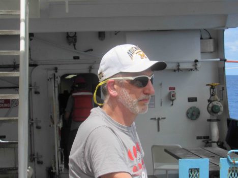
Andy Jessup, Chief Scientist on SPURS-2 R/V Revelle.
I would like to give a shout out to our chief scientist on the voyage, Andy Jessup, from the University of Washington Applied Physics Laboratory. Andy has demonstrated extreme patience and diligence to his duty to represent the many investigators working on diverse problems and scales in SPURS-2. He has a team from APL aboard with a complex set of measurements to execute. He balances the time devoted to his own science project and his duties as leader of all the projects represented on the ship. That is not easy and he has found a way to give everyone a voice.
I hope to devote some upcoming blog time to our able CTD crew from Scripps led by Janet Sprintall, the ocean currents in our region in general, and the interaction with the teams back home as seen through the eyes of Audrey Hasson.
Please feel free to send questions and comments on the blog. I’ll do my best to answer all fair questions!
As the first phase of the ATom project draws to a close, I am still surprised at just how far the influence of land, and fires in particular, can travel through the atmosphere.
Most of the time, the influence of land (and pollution that people generate) can only be seen a few miles from shore. When flying south into Alaska from the Arctic ocean, we saw the tell-tale chemicals of land influence about three miles offshore; uptake by plants reduced the amount of carbon dioxide (CO2) and increased the methane from emission from wetlands. Flying from James’ Bay in over the Hudson Bay Lowlands, we saw an even larger increase in methane a mile offshore than we saw in Alaska. I should not have been surprised, because Hudson Bay Lowlands are the largest source of natural methane in North America.
The Hudson Bay Lowlands in Canada are a large source of methane. Photo by Róisín Commane
But in other places we also saw pollution thousands of miles from shore, in amongst some of the cleanest air in the world. In fact, some layers of pollution were so concentrated that we could see them by just looking out the window. In the photo below you can see a brown/pink layer of pollution that we found hundreds of miles from land as it cuts through the beautiful blue sky and ocean below. In layers like this, CO, other pollution related gases and particles like black carbon will be pretty high. We saw pollution from Asia transported out over the Pacific ocean and pollution from the U.S. over the Atlantic ocean.
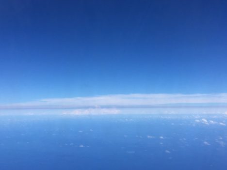
Pollution layers over the Pacific ocean. Photo by Róisín Commane
I’ve learned that pollution can be transported anywhere. The amount of pollution in the Arctic was especially stark. In Greenland we could see the black layers forming on the top of the ice sheet as pollution from far away gets transported to the arctic and deposits on the ice. The black layers absorb more heat than clean ice leading to increased melting at the top of the ice sheet, which forms deceptively beautiful melt ponds on the ice sheet. We met researchers from the UK “Black and Bloom” project (@BlackandBloom) in Kangarlussuaq and heard how some of this black layer can be composed of algae, which will also enhance warming and melting.
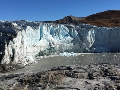
Russel Glacier near Kangerlussuaq, Greenland. Photo by Róisín Commane
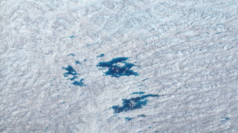
Bright blue melt ponds on the Greenland Ice Sheet. Photo by Róisín Commane
However, not all pollution is man-made in the typical sense. In the Arctic regions north of Alaska and Greenland, which we sampled almost three weeks apart, we saw the high carbon monoxide (CO) given off by the fires in Siberia. Fires in this area are a part of the natural cycle, but as temperatures have been rising in the Arctic, the frequency and magnitude of big fires like these have increased. In Alaska last year, over five million acres burned. In Canada the year before 11 million acres burned. These regions have carbon rich soils similar to dry peat bogs, that often continue to smolder and incompletely burn long after the hot temperatures of the main burn. Lower temperatures and incomplete burning leads to the release of more CO, soot and other pollutants than for a hot, completely burning fire.
The arctic regions are not the only place we see the influence of very distant fires. We sampled air from fires burning in Africa as we came into land in Ascension Island. As the Island is 1,000 miles from any continent, I was really surprised that the high CO could survive that journey! CO has a lifetime of about a month in the troposphere, and some of the other chemicals are much shorter, so the air has to travel to remote islands like Ascension fairly quickly.
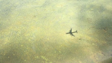
I’m often a little torn by seeing layers of high pollution in the remote atmosphere. While it’s exciting to see high numbers on our instruments, it’s really disappointing to think that the places we think of as pristine see so much human influence. But any time I get a little down, nature has a way of cheering me up: such as when the sun and clouds combine to create a glory around our aircraft. You can tell from where the glory is centered that I was sitting just behind the starboard (right) wing of the aircraft as we ascended through the cloud layer. A glory forms around an aircraft when there are clouds (or water) in the air and the sun is directly behind the aircraft.
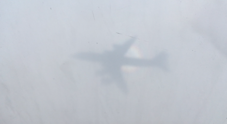
The shadow of the DC-8 on clouds below, haloed by a “glory”. Róisín Commane
The ATom mission is the first to traverse the whole lengths of the Atlantic and Pacific Oceans while making atmospheric measurements from the ocean surface to high altitudes. When we planned ATom, one idea was to compare pollution impacts between the oceans. I expected that human activities would have much greater influence in the Atlantic, because it is smaller than the Pacific and it receives industrial emissions from both sides – the U.S. on the west and Europe to the east. The big emissions from Asia appear to go north to the Arctic, mostly bypassing the Pacific.
Already, our measurements have shown me that our notions did not always match reality. The North Pacific was full of pollutants from Asia, but not from industry as we might have expected—they came mostly from forest fires in the Arctic. Near the coast of California, we did see industrial pollution, but even there, the impact from the large forest and brush fires raging through the Western U.S. this summer was much greater.
So we departed New Zealand and flew to Punta Arenas, Chile, across the tempests of the Southern Ocean off of Antarctica. We found the cleanest air we encountered anywhere, although even there, we could detect very faint traces of soot and other combustion products. It was windy, snowy and cold in Punta Arenas.
Crisp air had arrived from Antarctica, by the time we embarked two days later for the Atlantic. It was just as clean as it looked.
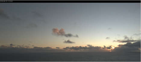
Crisp, clean sunrise seen from 500 ft over the South Atlantic east of Argentina. Photo: NASA DC-8 forward camera.
We headed from Punta Arenas to Ascension Island, a small, isolated, mostly barren volcanic protrusion emerging from the very center of the Atlantic at the Mid-Atlantic ridge, where the ocean basin is created, 12 degrees south of the Equator. It is extremely remote, more than 1000 miles from the nearest land.
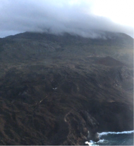
Ascension Island, our destination in the middle of the tropical South Atlantic. Photo: Steven Wofsy
An hour or so after leaving Chile, we crossed the frontal region of stormy weather that separates the wintry middle latitudes from the subtropics and tropics in the south Atlantic—the southern polar jet stream. Air quality started to deteriorate immediately after we had crossed the jet stream, and pollution got stronger and stronger as we approached Ascension. By the time we arrived there, smoke and haze were so thick we could not see the surface of the ocean looking down from above. Here we were — actually dead center in the middle of the ocean — and pollutants from brush and forest fires in Africa were as heavy, or heavier, than the smoke and haze we encountered when we started out in Palmdale, California, where there was a large brush fire nearby and the City of Los Angeles just upwind!
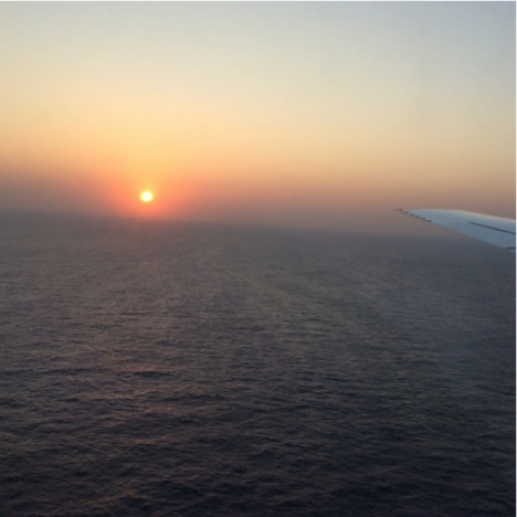
Dense smoke and haze obscure the sunset as we approach Ascension Island, in the center of the tropical Atlantic Ocean. Compare this image with the sunrise that we observed on departing Chile! Photo: Steven Wofsy
I was not surprised to find pollution at Ascension, its presence had, once again, been forecast by our modelers, Junhua Liu and Sarah Strode from Goddard Space Flight Center. But I was stunned at how dense and extensive this pall of haze and noxious gas was. We found quite a bit more than what the models predicted. No wonder we had earlier seen African pollution way out in the Pacific, 3/4 of the world away from the source!
We had wonderful hospitality from the U.S. airbase on Ascension, but this part of the trip was really discouraging. The rocky little island was inhabited by all manner of invasive species—plants, rodents, feral livestock, etc. The accommodations were spartan, and we were mostly cut off from communications with the outside world. The air that we came to study was a mess. We had traversed 12 time zones in a few days, so our bodies wanted to sleep when we needed to be awake and vice versa.
We were thankful to our gracious hosts, but ready to move on to our next destination, Lajes Airfield on Ihla de Terceira in Portugal’s Açore Islands. On this leg of our trip, we crossed the Intertropical Convergence Zone once again. On the north side, there was still a lot of pollution from African biomass fires and a good dose of Saharan dust, too.
We arrived at Lajes just after a storm had passed through, putting us in air from middle latitudes. The air was much cleaner. We stayed at a quiet town, Praia da Vitoria-Santa Cruz, on Ihla Terceira, with comfortable lodgings and excellent restaurants that emphasized local seafood and produce. It reminded me of the fresh-as-ever cuisine of Provence, France. I slept a lot, and enjoyed the place thoroughly.
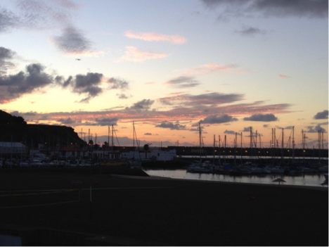
Praia da Vitoria-Santa Cruz, Ihla Terceira, Açores, Portugal, at sunrise. Photo: Steven Wofsy
But I admit to having had a feeling of unease. The atmosphere over the Atlantic was far more polluted than I had imagined, and a large fraction of the whole ocean was being affected.
Nevertheless, I came away refreshed and invigorated after two days in the Açores, and I think the whole crew felt renewed and eager for the final legs of our journey—on to Greenland, ground zero for climate change.
