Walt Petersen is the Ground Validation Scientist for the Global Precipitation Measurement (GPM) mission, based at NASA’s Wallops Flight Facility in Virginia. He manages all of GPM’s ground validation operations, the field campaigns that ensure that satellites measure rainfall and precipitation from space accurately.
From May 1 to June 15, he is leading the Iowa Flood Studies, or IFloodS campaign in eastern Iowa. He and his team, as well as their partners at the Iowa Flood Center at the University of Iowa are measuring rainfall with ground instruments, ground radar, and satellites, and then evaluating flood forecasting models. Over the next few weeks, Walt and others on the ground will be sending us their notes from the field.
4/29/2013, NPOL Radar Site near Traer, Iowa

Apr 29, 2013. The NASA Polerametric (NPOL) precipitation radar (center) scans for rainfall in both the horizontal and vertical planes to measure precipitation throughout the whole volume of the air column. The smaller D3R radar is to the far left. Credit NASA
This morning, my first full day around the area of Waterloo, Iowa. Quite appropriately, we were greeted by severe thunderstorms with some ping pong ball-sized hail in the area. Luckily for my rental car, and even more luckily for the NPOL and D3R antennas, that hail stayed north of the radar site (large hail, rental cars, and/or radar antennas not being the best mix). I thought it an appropriate welcoming to the experiment. I drove out to the radar for the first time this morning in my little Nissan rental car. I’ll be curious to see how it does on the gravel/dirt road after it rains a few inches.

Apr. 25, 2013. A team of NASA staff and Iowa Flood Center and University of Iowa students assist with the NPOL setup in eastern Iowa. Credit: Aneta Goska, Iowa Flood Center.
Things are impressive out here. The NPOL and D3R guys did a very nice job of getting the NPOL and D3R set up. We are still in the midst of tweaking small things prior to getting down to serious data collection. For example, we need to make certain that the NPOL is well-calibrated (doing that now), and then we need to test the timing of our scan sequences to make sure we are making the requirement that we sample the rain field in a 360 degree circle once every 3 minutes or less. The objective is to make rapid maps of rainfall (out to a range of say, 150 km, from the NPOL) at high time and space resolution, and then in between making those rain maps, do coordinated scanning of the precipitation in the vertical plane with the D3R radar or over other river basins of interest. The rapidly collected rain maps serve as a reference for doing our comparisons to satellite products and to test products for hydrologic modeling of runoff (e.g., flood forecasting).

Apr. 29, 2013. The science trailer where data from the radars is collected. From left to right, Walt Petersen, Dave Wolff, and Delbert Willie. Credit: NASA
The coordinated scanning with the D3R is done for a slightly different reason. These scans are collected along a line that has many raingauges and disdrometers located at different points so that we can connect the dots between the rainfall we are measuring near the ground (for example, rainfall rates and raindrop sizes, numbers and shapes) to the physics happening in the column of the atmosphere above those points (e.g., how the rain is made). We care about this from the perspective of testing algorithms designed to retrieve precipitation estimates from space using the GPM DPR radar (which has similar frequencies to the D3R) which will fly on the GPM Core satellite.
By Clément Miège
Hi there! Today I have another story to share with you! It’s about the tracking of the temperature evolution of the firn aquifer temperature by using two thermistor strings that we set up in the two holes made by Jay (see Jay’s post on drilling for details).
By tracking temperatures over a year, we will observe the firn heating mechanisms in the summer with the melt from the surface of the ice followed by water infiltration in the firn. In the winter, we will get a sense of the refreezing processes from the cold surface air, which cools the upper part of the firn and we will observe the persistence of the firn aquifer over the years.
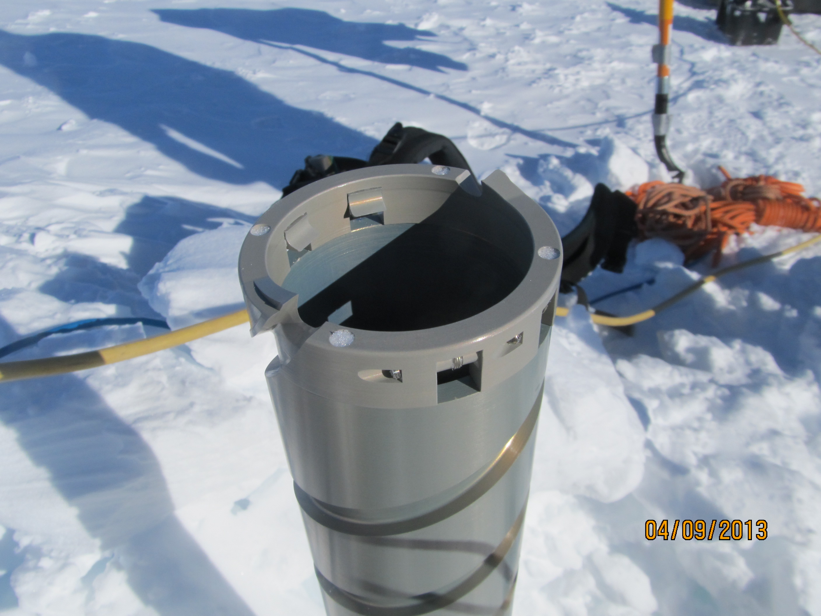
To achieve this, we installed two thermistor strings with two different lengths: 30 and 60 meters. The shorter string has 60 sensors on it, sampling every half-meter. The longer one will only get a temperature reading every 2.5 meters but it will record deeper temperatures. Both strings are set to collect data every hour for an entire year, assuming the batteries last that long (hopefully!) The temperature chain is called a thermistor string because each sensor is a thermistor, a type of resistor sensitive to temperature changes. After measuring a resistance change, calibration curves allow us to retrieve temperature changes.
The thermistor-string story started in Utah, when we received the equipment late from the manufacturers, giving us only 5 days to work on it before leaving for Greenland. We realized that integrating the whole system together with the satellite uplink would take most of our last prep days.
It was definitely too late to ship the thermistor equipment with the rest of our gear, so Rick and I traveled with it in our checked luggage! I ended up with a 50 lbs of spool coiled with about 60 meters of cable in a suitcase. Rick had a black pelican case as his checked bag, with the second thermistor string, datalogger, ARGOS antenna and other pieces of hardware. We learned how to travel light, bringing minimal clothing, and wearing the cold-weather clothes in the airplane so we were able to meet the airline luggage restrictions – it definitely made for fun travels!
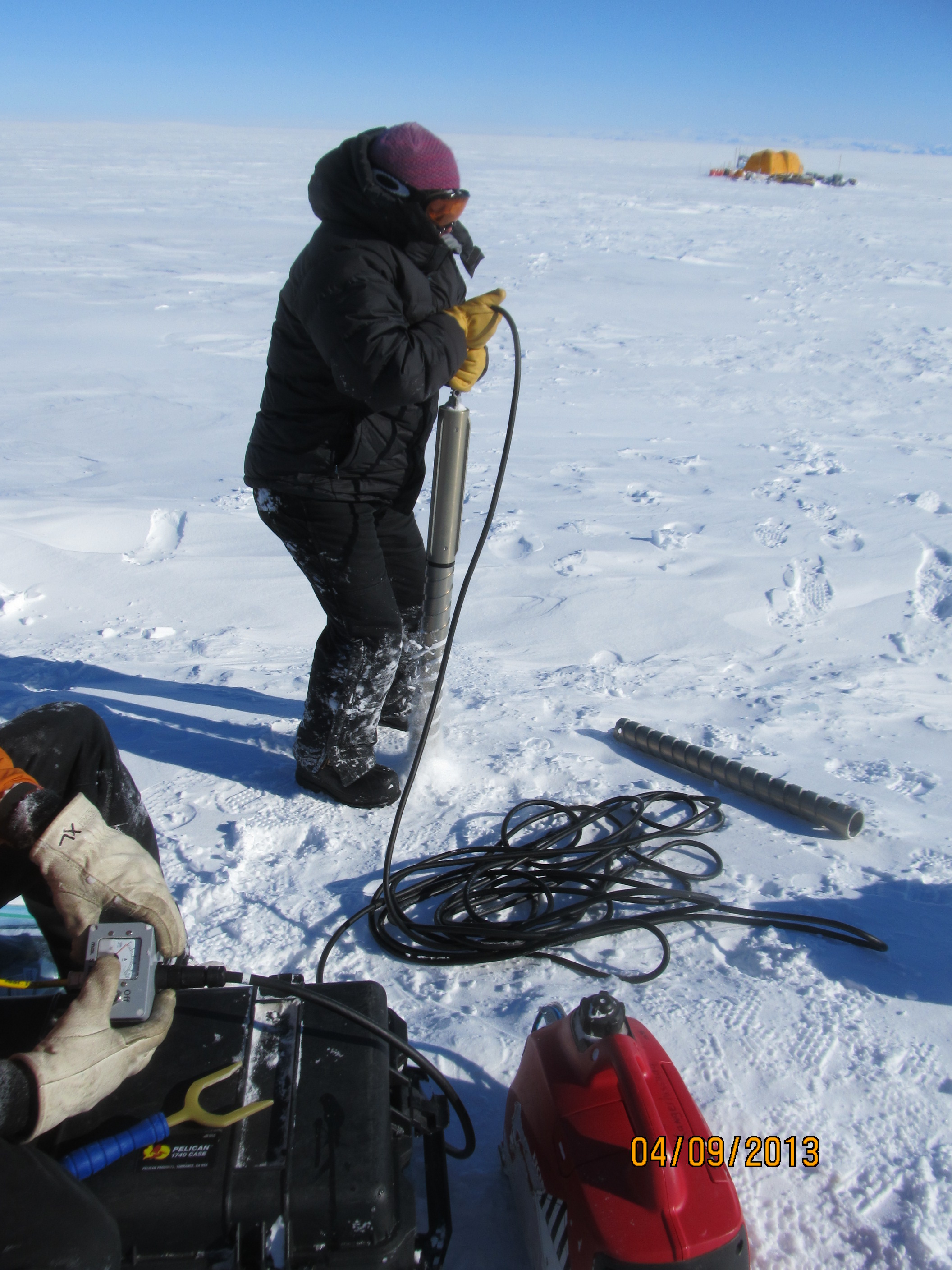
At the Kulusuk Hotel, in southeast Greenland, we finished integrating the thermistor string, mostly by picking the right data-transmission rate to the satellite in regards to our battery consumption estimates. Having the ARGOS satellite uplink will let us receive temperature data via email every day from the field site and tell us almost in real time what the temperatures are in the two holes.
In the field, shortly after drilling each hole (to avoid water refreezing due to cold air down the hole), we lowered the thermistor string down and backfilled the hole with surface snow. Then, we used the Felics drill to make a 4-meter hole to anchor the long pole that holds the ARGOS antenna.

Lowering the second thermistor string down the 30-meter hole.
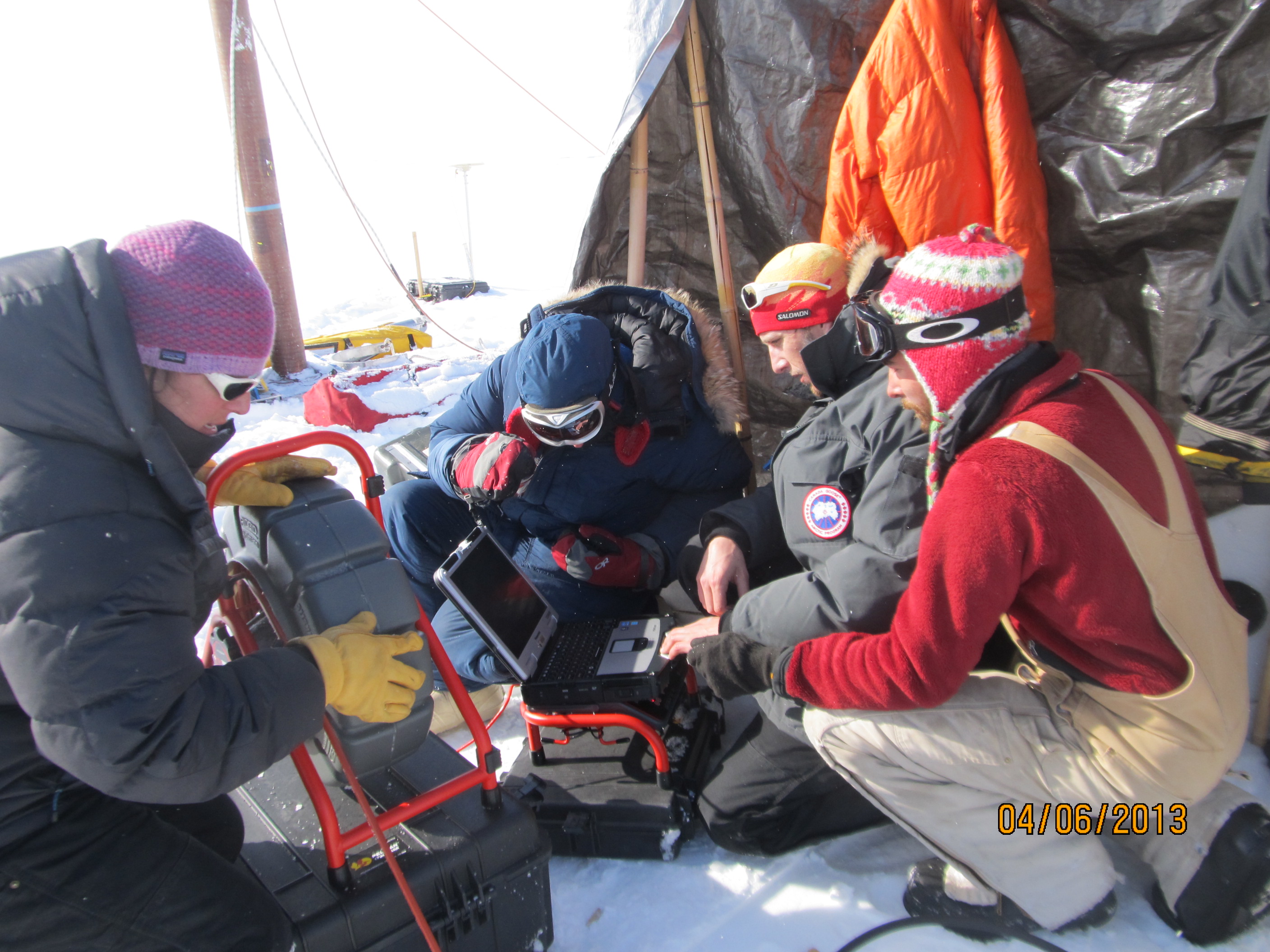
On that day, the 20-knot katabic winds were blowing a lot of snow, so we used a mountain tent as a snow-proof environment to work with the electronics before dropping off the case in its hole. To give you a taste of the wind speed: Rick was charging one of the thermistor-string battery and the wind was so strong that it blew the small 1kw generator off…. crazy! When the winds finally died down, we buried the case in a 2-meter deep snow pit, because we wanted to prevent the case from being exposed to surface densification and melt during the summer.
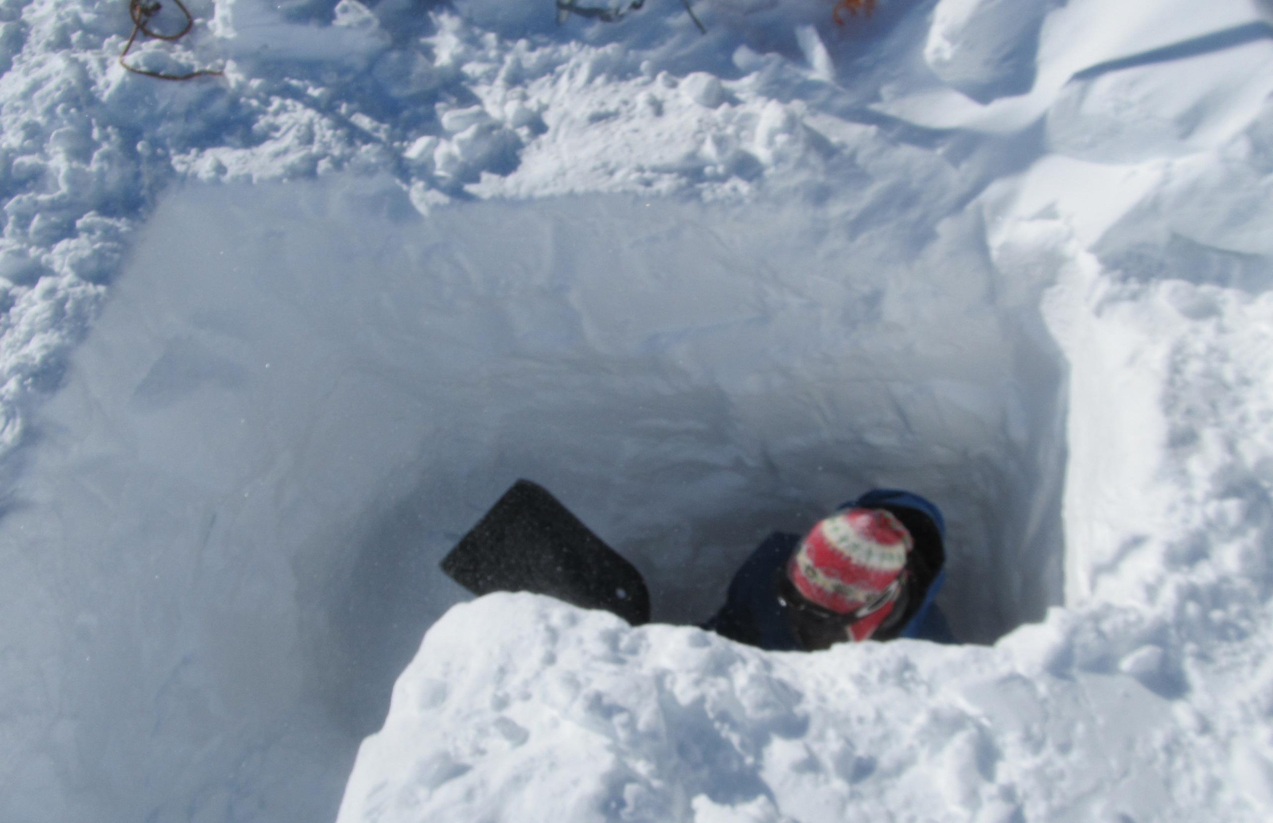
Digging a deep snow pit for the thermistor case.
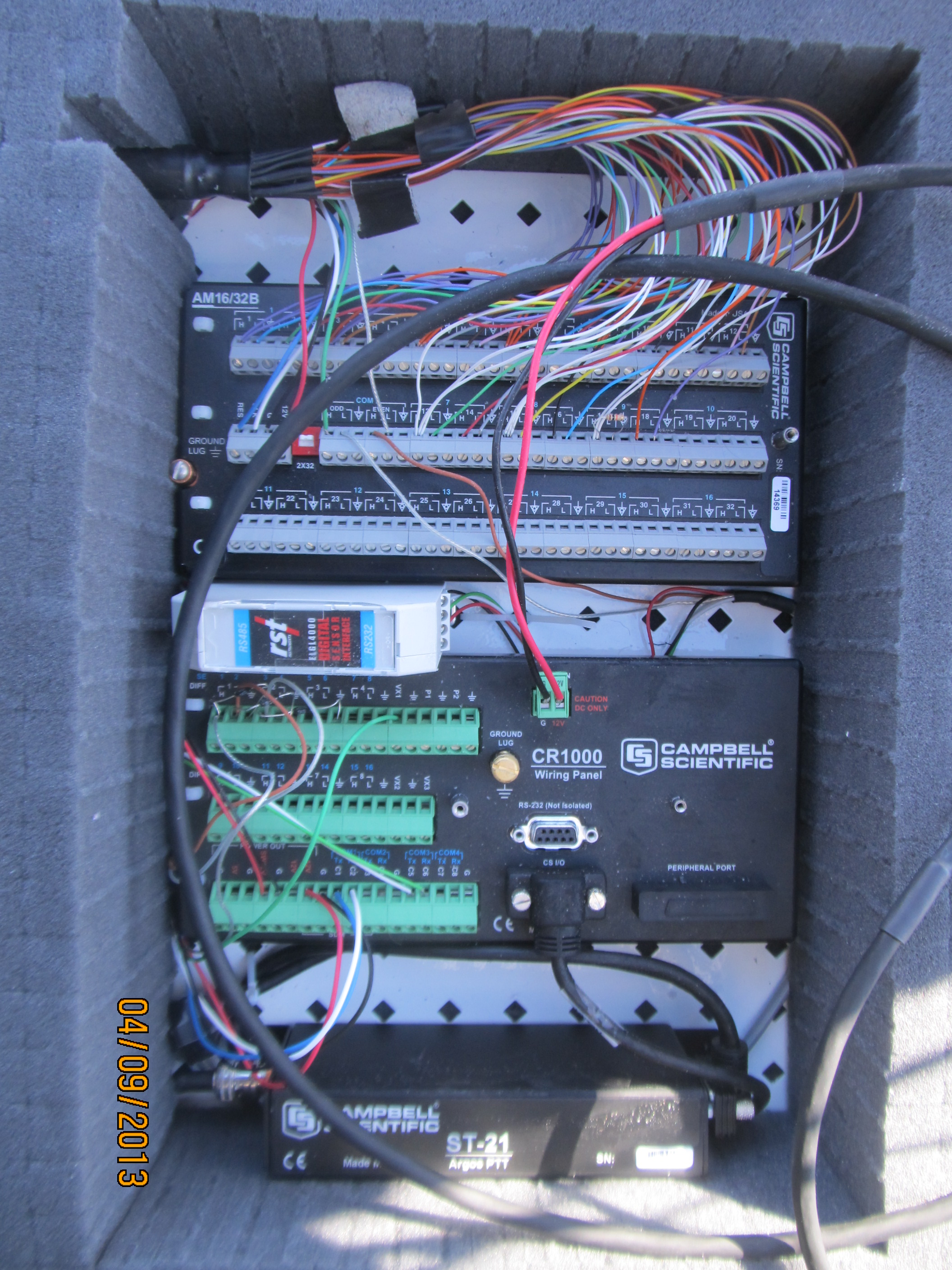
Last check on the electronics, to make sure all the wires are tightened before closing the box — next opening in one year!
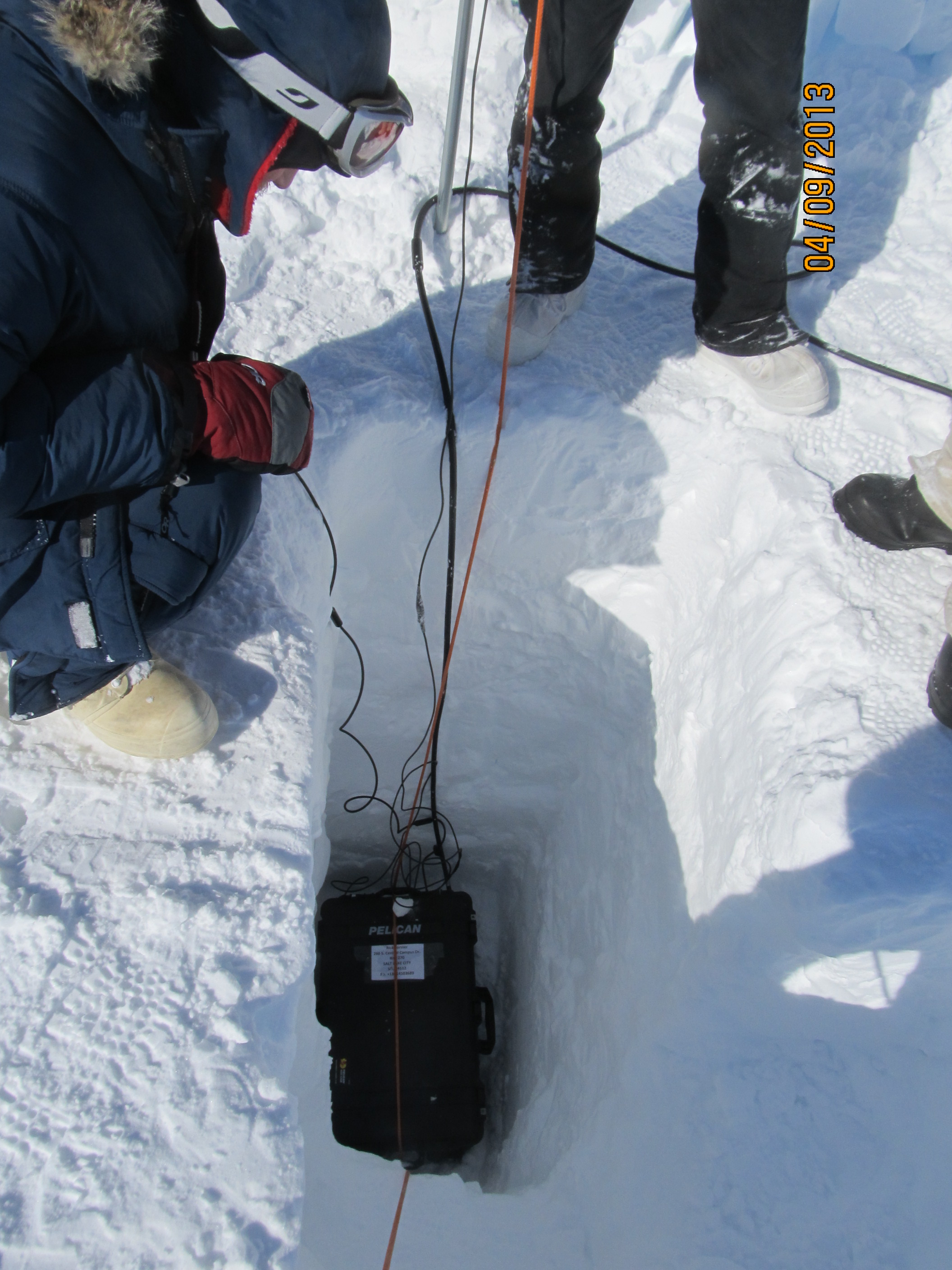
That is it! The box is down the hole.

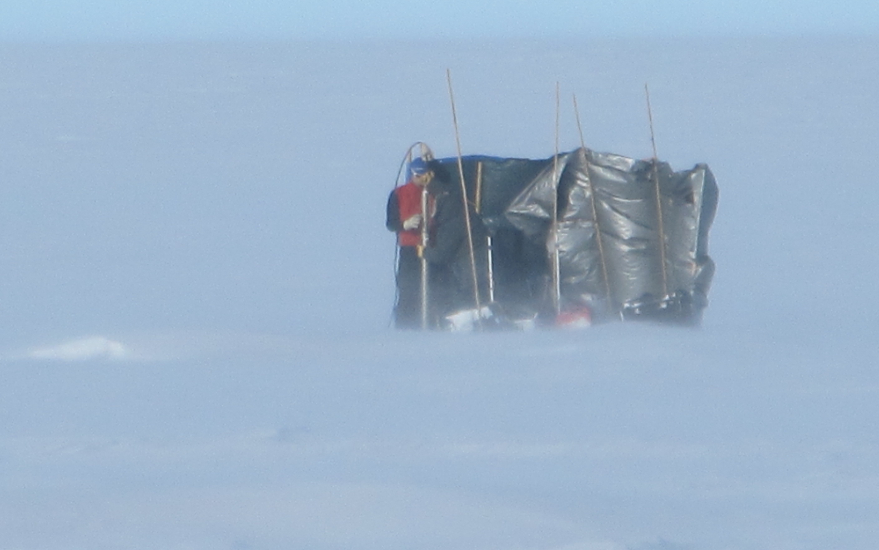
After backfilling the snow pit, the only evidence at the surface of the temperature strings is the top of the pole with the ARGOS antenna and a red flag!
We are hoping to recover the case with the datalogger next year, but we are not sure if the ARGOS antenna will still be sticking out, because this sector of the ice sheet is getting a lot of snow accumulation in the winter. We will use a metal detector to find the metal pipes left near the case.
Because this is likely my last post for this expedition’s blog, I would like to thank the all team for this great adventure and everybody that was supporting this exciting research. Until next time!
By Lora Koenig
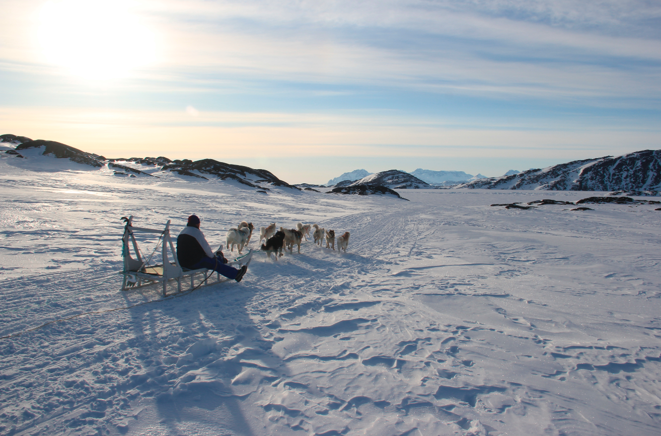
Watching dogsleds go by in Kulusuk.
Well, I am back in Greenbelt, Maryland, typing with warm fingers in a climate-controlled office with high-speed Internet and drinking fountain just down the hall. After fieldwork, I am always thankful for things I generally take for granted, like being able to charge my laptop by simply plugging it into an outlet. There is no longer a need fill a generator with gas and then start it just to charge batteries. Aw, the comforts of home! (We all had safe trips back to the US and have returned to our home institutions last week.)
For the last blog post of the season, I decided to pull together a few of my favorite photos from our trip to give you a sampling of the great fun we get to have while doing this kind of research. The most fun I had during this trip was on our final day in Kulusuk: we were invited to the Kulusuk School to with the children in the upper grades (who speak some English) about our work. I regret that we do not have any pictures of this event, but we were giving our presentation and letting the students run our small ice core drill, thus neglecting picture taking. The school in Kulusuk has about 70 students and includes all grades. The building has lots of windows and is very bright inside — it is one of the prettiest schools I have been in, with lots of open space, a small kitchen, library and a gym. I especially liked the entrance to the school, which was equipped with plenty of coat hangers and boot racks for the students to shed their cold weather gear as soon as they come inside. Though we were there talking about science, the school in Kulusuk is known for their art. We were hosted by the art teacher, Anne-Mette Holm, and after our talk got to attend one of her classes where the students were making wooden sculptures. We also got to see other student projects including weaving, toy making and furniture making. Quite a portfolio! The students’ art has traveled the world, being shown at different expeditions across the Arctic. (Check out pages 11 -15 of this document for some examples of the children’s art work under Anne-Mette’s tutelage.)
While our visit to the school was definitely the top highlight of the trip here are a few others highlights in pictures.
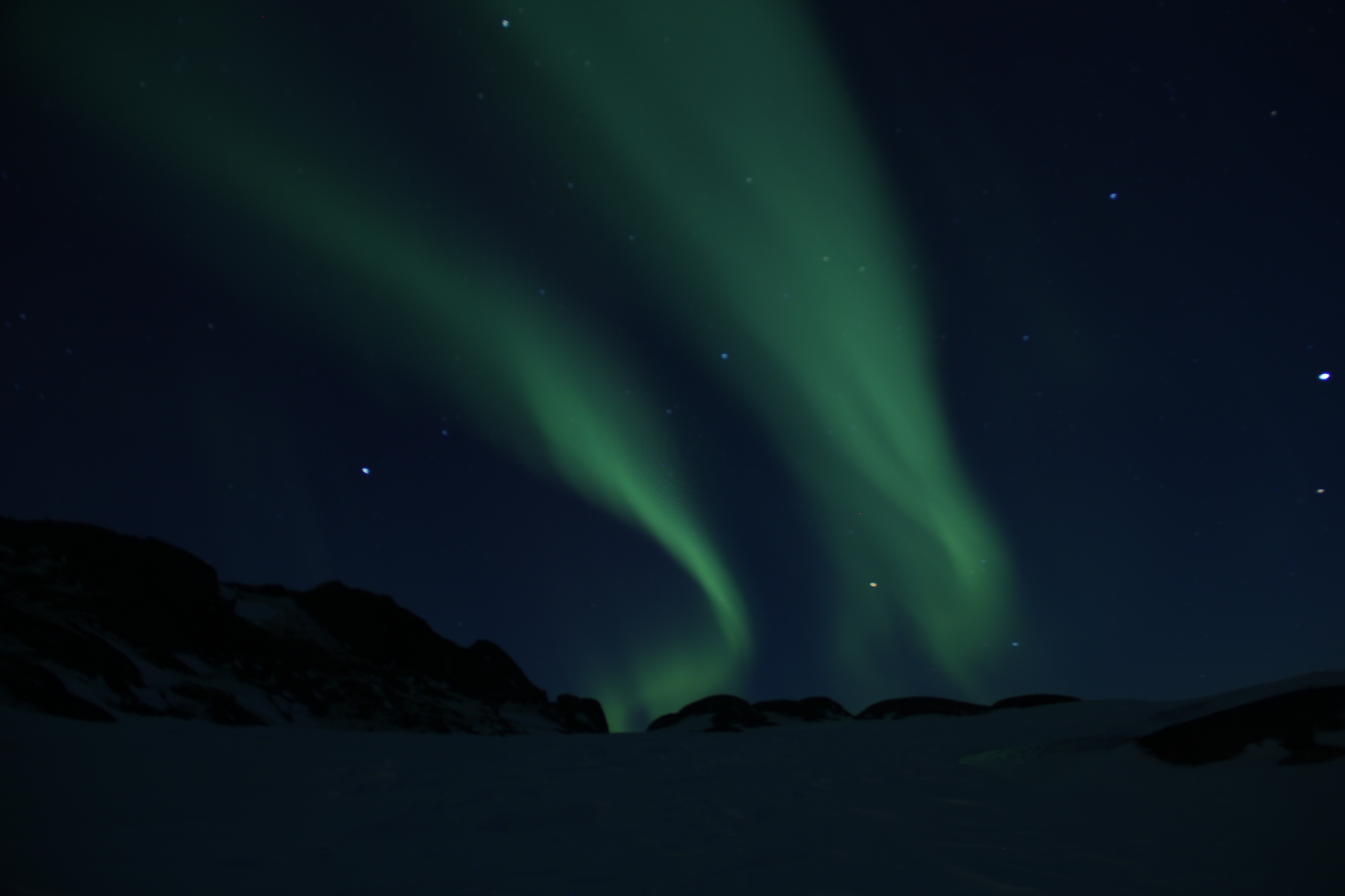
The northern lights (Aurora) never got old and were out almost every night.

The view out the window from our dinner table in Kulusuk at sunset.

Sunset in Kulusuk.
Seeing mountains from our campsite on the ice sheet, a nice change from the typical flat white ice sheet.

Watching Clem dig a really big hole for the thermistor control boxes.

Seeing the transition between the flat ice sheet and the fast flowing outlet glaciers.

Catching a ride in the airport luggage carts.
So those were some of the highlights of the field work and now it is time to work with the data we gathered. In the week we have been back, we have already started to analyze our data. We see that, as expected, the densities in the firn (aged snow) above the aquifer are higher than expected and that there is more water than originally predicted. We still need more data to fully understand what this water trapped in the Greenland ice sheet means for sea level rise. We need many years of data to understand how and if the aquifer is changing with time… but remember this was an exploratory mission. When we set out, we were not even sure if our drills would even work. There was a chance they would have just frozen in place and we would not have gotten any data. This was a high-risk mission due to the weather in the region and all the new things we were trying. We came back with all the data we set out to get and, quite frankly, I am surprised. We had a large team that helped with this project including the field team, logistics support, airport support, the NASA and NSF support teams and all of you for your well wishes and interest in our research. Thanks to all! Until next time, stay cool 🙂
By Ludovic Brucker
We were on Greenland’s ice sheet for only a week, but despite the short deployment, we had to accomplish two main science objectives. The first was drilling two deep cores into the firn (aged snow) and ice (30- and 65-m deep, respectively), to insert temperature probes that will record temperature evolution at various depths. Secondly, we wanted to drill shallower cores (7 to 15 m) to record the snow’s density vertical profile using a neutron density probe – and this is what this post is going to be about: the shallow drilling that we did and the measurements we took in these holes to monitor the snow and ice layering and their properties.
To drill the shallower cores, we used the same solar-powered drill as in 2010 and 2011 in Antarctica during the Satellite Era Accumulation Traverse. It is composed of four parts, which I’ll describe from top to bottom. The first segment contains the motor to rotate the other parts. The second and third parts are barrels — one for the snow and ice chips, and the other to store the one-meter long drilled core. The fourth part, the cutters, is screwed into the latter barrel. Cutters are critical since they are the sharp elements that cut the snow, firn, and ice. Since snow and ice having different properties, the cutters for snow and ice are different. For instance, if we use the ice cutters at a smaller angle, we will drill at less depth during each barrel rotation. Where we drilled, part of the winter snow melts during the summer and when it refreezes, it forms a thick ice layer every year. The snow that did not melt will slowly evolve to firn, and, eventually, ice. Because of the different, we thus had to switch cutters during our drilling: otherwise, we would have not been able to drill through the past summer ice layers.
Ice cutters screwed at the bottom of the barrel, which rotates into the ice to extract an ice core.
Lora showing how to extract the first meter of the snow core.
Jay drilled cores through the water contained within the firn (the aquifer). We used our smaller drill, since we did not want to enter in contact with the aquifer. Therefore, each of our cores was shallower than the water layer’s top and each was drilled in about an hour.
Once we had drilled the hole, we observed the layering of the snow and ice cover using a video camera. Thanks to the camera’s flashlight, we were able to identify the thick 2012 summer ice layer (about 3 m below the surface) that formed after a massive surface melt event, as well as the previous summer ice layers. Our team used this sensor to monitor a water-filled hole for the first time. We were all really excited to see the inner upper part of the ice sheet!

Lora holding the video camera that she will send down in the hole to monitor the snow and ice layering.
Rick and Clem enjoying the first view of the firn’s internal stratigraphy
We also used this useful device to check the position of the temperature probes and to ensure that the entire line of temperature sensors was straight inside the hole. The first time we inserted the camera into the water in the hole, we were amazed to discover the amount of air bubbles released by the firn, which propagated toward the water/air interface. The aquifer is composed of ice, water, and air. These elements are present several meters below the surface, which means they’re under pressure. Once we drilled the cores, the pressurized air bubbles in the vicinity of the hole migrated toward the hole and then moved upwards to the water/air interface.
Our last scientific activity was to monitor density with 1-cm vertical resolution using the neutron density probe. We moved the probe along the borehole at a speed of about 5 cm per minute. This sounds like a time-consuming measurement, but measuring density manually is significantly more labor intensive since one must saw the core into segments and then measure each segment’s length, diameter, and weight.
To be more comfortable during the drilling and while recording our scientific data, we always paid particular attention to staying behind our wind break.
Lora and Ludo drilling behind a windbreak during a windy day, with a lot of blowing snow near the ground.
A windbreak is composed of a simple plastic tarp supported by bamboo sticks and held by bungee cords. While we were in Kulusuk preparing our departure to the field, Jay told us several times that bamboo sticks would be critical pieces of equipment while we worked on the ice and that they had to be in mint condition to offer the best resistance to wind. So we spent more than a day in Kulusuk fixing and reinforcing bamboo sticks, using wires and tape. And I am glad we did it!
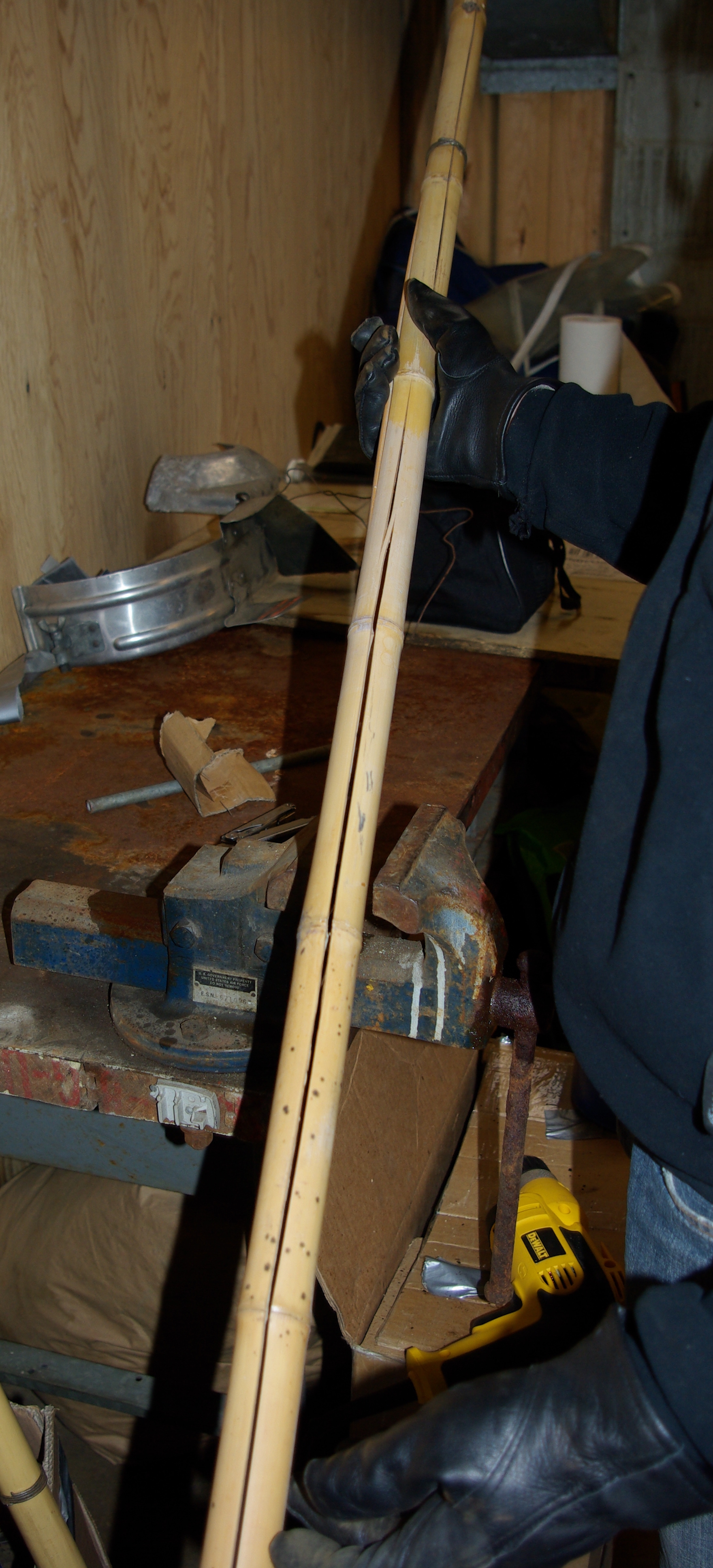
Working in the warehouse to improve the bamboo sticks that we’ll use in the field as wind breaks.
Once we had collected all the data needed from a hole, we packed our equipment, removed the precious windbreak and the bamboo sticks, and either headed toward a new site few hundreds meters away, or went to the cook tent for diner. That’s how our busy days in the field went!
By Clément Miège
Hi there! Today I will give you some background on the radar measurements we collected in southeast Greenland. The radar we deployed is sensitive to snow density changes and to wet snow. The main goal of the radar measurements was to provide information about the spatial variations of the top of the aquifer (a water layer trapped within firn, or old snow).
The radar we used is made by GSSI, a company specialized into geophysical measurements, and it has a center frequency of 400 MHz. In snow and firn, the electromagnetic waves sent by this ground-penetrating radar can image approximately the first 50 meters of a dry snowpack. The layers that we observe in radar measurements show the snowpack stratigraphy (density changes). If there is water within the snow and firn, we observe a really strong radar echo in the radar profile. Then, by dragging the radar around, we are able to see how this water layer evolves spatially.
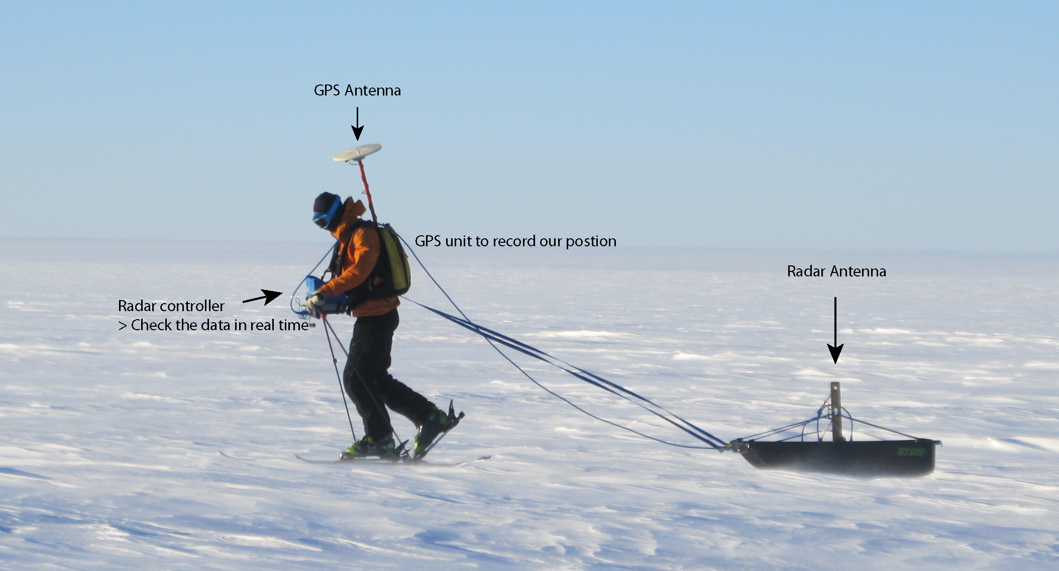
Here is the radar system in action, with Ludo pulling the sled. It can be a pretty tiring job with the wind and the cold. The balaclava was an absolute must to protect your face from the freezing temperatures.
Mostly to lighten our helicopter loads, but also to exercise a bit, we decided to pull the radar sled with skis. But it ended up not being an easy job at times: some of our field days were really windy and cold, so we needed to be warmly dressed and have our face well-protected. In addition, we carried a backpack with the GPS unit and a battery – they became pretty heavy after an hour of pulling the radar. Ludo and I set up the rule of not doing more than 2 hours of survey at a time, which corresponded to about 5 km total.
Once on the ice sheet, as soon as the helicopter took off, we turned on the radar. Indeed, we wanted to make sure that we had been dropped over water and then find the best location for our drilling site. By looking at the radar profile, we identified the water layer (great!) and we converted its depth from electromagnetic wave two way travel time to meters. We observed that over a 2-km transect, the top of the aquifer varied up to 10 meters. By knowing this variation, we were able to pick the site location at a depth that fitted our science needs.
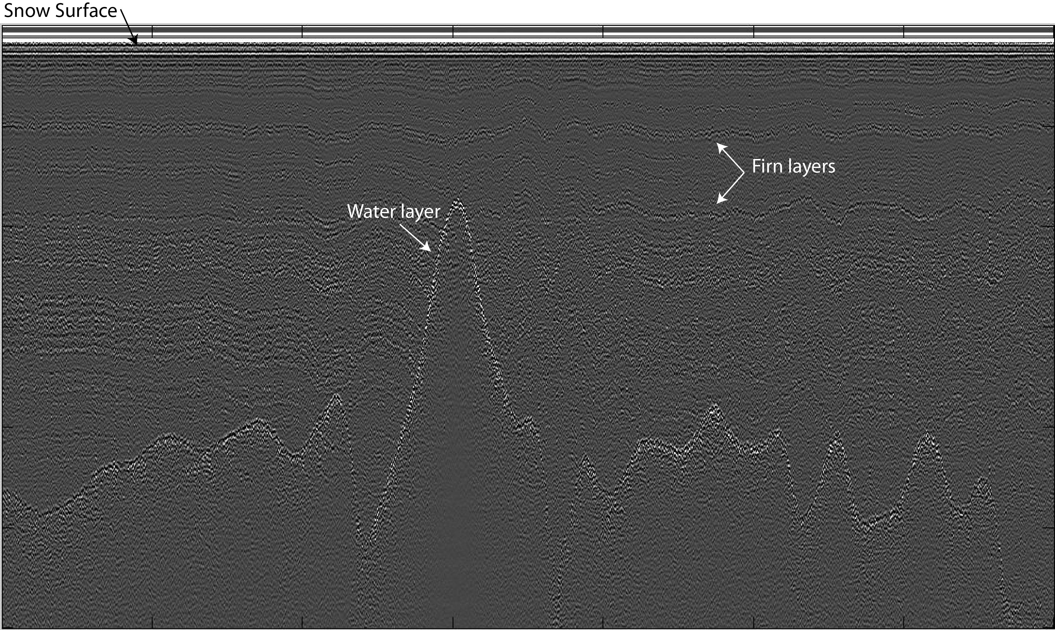
An example of the radar profile observed: the bright reflector represents the top of the water layer. Other internal reflections can be seen — they are linked to previous summer layers, which are denser.
The advantage of doing this preliminary radar survey is that we then knew before drilling at which depth the drill would encounter water and penetrate into the aquifer. And the good thing was that the radar picked the right water depth in both drilling sites! The radar ended up being a really good tool to extend spatially the localized information obtained by the firn cores.

Doing some radar at sunset with no wind was just so great!
For the radar survey, we were doing some elevation transects, to see how the water layer changed with the local topography, and some grids and bowties to extent spatially the core site stratigraphy. We stayed within a radius of 2 km from our camp.
Overall, doing the radar surveys was a great experience. It’s incredible to think that we were skiing with liquid water right below us, while surface temperatures averaging -15C.
Finally, concerning the radar setup, we have already some improvements in mind for the next time. For example, the GPS unit and its antenna need to be in the sled, maybe mounting the GPS antenna on a corner of the radar sled, trying to keep the all setup stable. That will allow us to drag the radar longer. We will work on that for our next radar adventure!
