Very few people get to fly 65,000 feet above Alaska’s glaciers. And even fewer get to fly over ones they share a name with. But on Friday, as pilot Denis Steele flew NASA’s ER-2 aircraft from Palmdale, California, to Fairbanks, Alaska, he snapped a picture of the scenery below – including Steele Glacier in the southwestern corner of Canada’s Yukon territory.
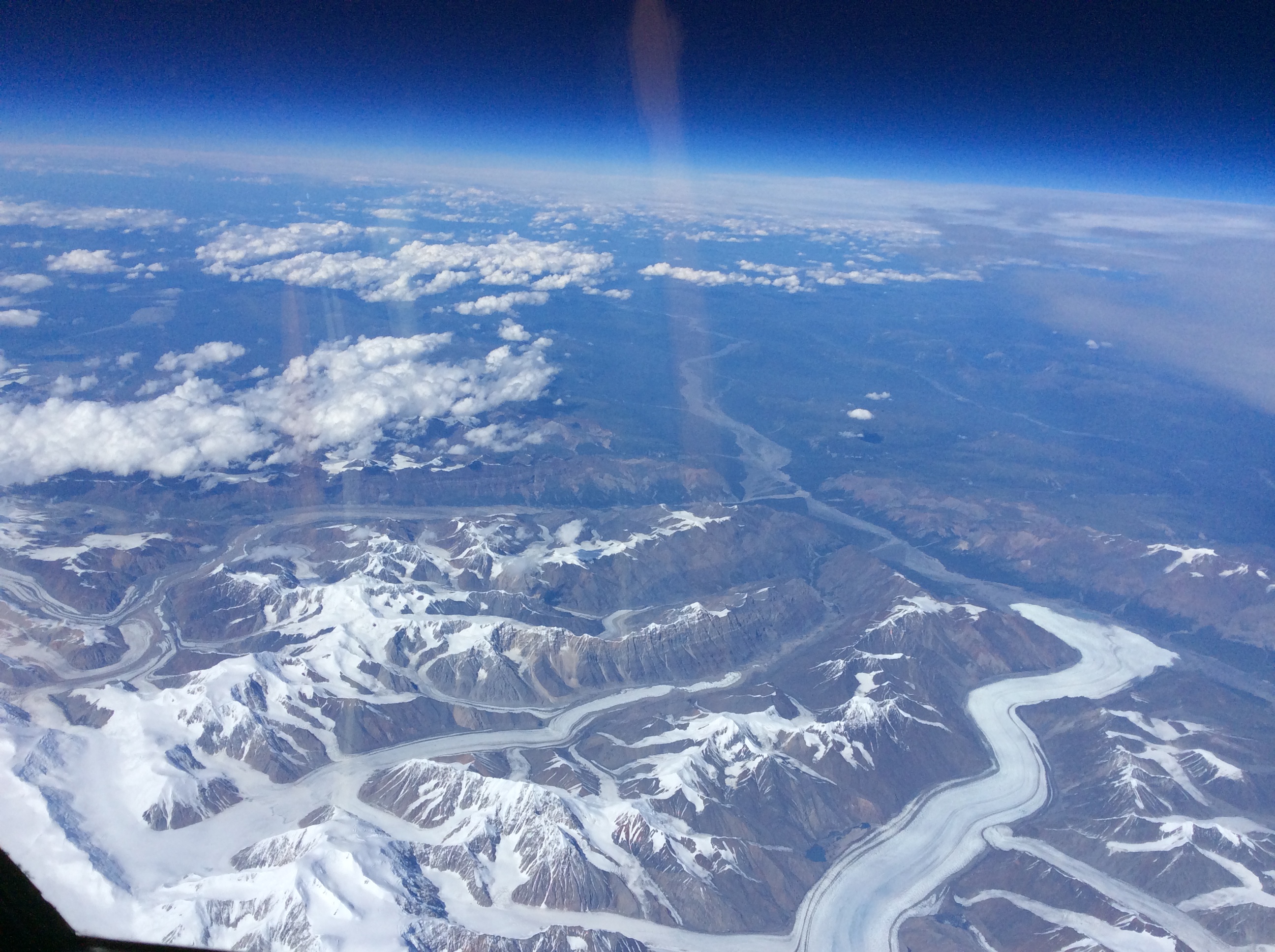
From NASA’s ER-2 aircraft, pilot Denis Steele saw glaciers in southern Alaska and Canada — including the Steele Glacier, the horizontal feature in the center of the image, and the Donjek Glacier (lower right). (Credit: Denis Steele)
Steele and the ER-2 team, along with NASA scientists, engineers and others, are here in Fairbanks to fly a laser altimeter – MABEL, or Multiple Altimeter Beam Experimental Lidar – over melting summer sea ice, glaciers and more. It’s a campaign to see what these polar regions will look like with data from ICESat-2, once the satellite launches and starts collecting data about the height of Earth below. Gathering information now allows scientists to get a head start in developing the computer programs scientists will need to analyze ICESat-2’s raw data.
MABEL and other lidar instruments are flying on the ER-2, which provides a high-altitude perspective. In the next three weeks, the plan is to cover melting sea ice, glaciers, vegetation, lakes, and more.
Steele wasn’t the only one looking out of the plane windows on flights north. Kelly Brunt, a research scientist at NASA’s Goddard Space Flight Center, spotted a wildfire in Eastern Washington. The fire, burning in steep terrain, resembled an erupting volcano.
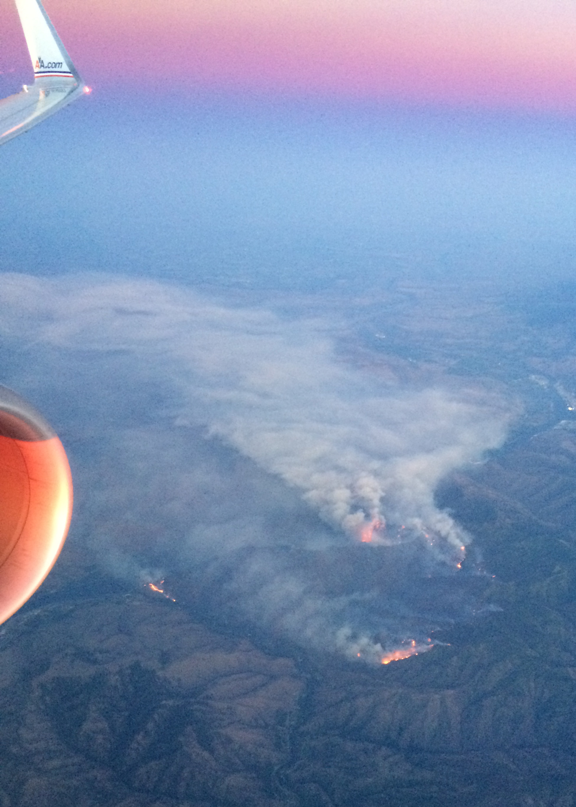
A wildfire burns in Washington, just east of the Cascades. (Credit: Kelly Brunt)
Over the weekend, the team settled into Fairbanks and a hangar at the U.S. Army’s Fort Wainwright, downloading data from the transit flight and ensuring the instruments are ready to fly when the weather allows. Cloudy skies over key sites means the ER-2 won’t fly today (Monday), but the team will check the weather tonight and see if it clears enough to fly the first science flight on Tuesday.
Want to follow MABEL and the ER-2? Check back here, and also check NASA’s flight tracker: http://airbornescience.nasa.gov/tracker/
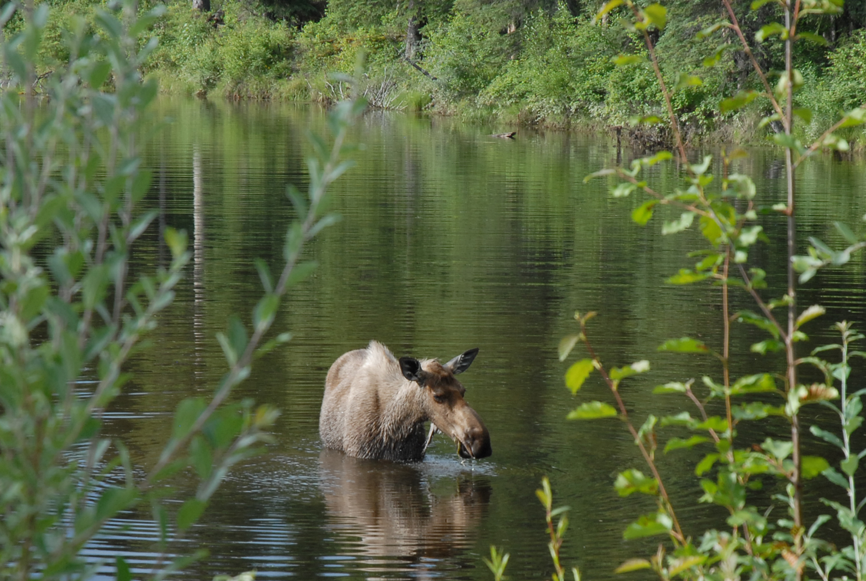
Yep, we’re in Alaska! A moose along a road east of Fairbanks. I’ll call her Mabel. (Credit: Kate Ramsayer)
Welcome to the LARGE (Langley Aerosol Research Group Experiment) blog. We are a group of scientists at NASA Langley Research Center in Hampton, VA who study the chemical, optical, and microphysical properties of atmospheric aerosols and their effects on climate and air quality. We are involved in many exciting experiments with vastly different objectives and applications, but this blog will begin by focusing on a project this summer/fall to assess the distribution and impacts of aerosols on hurricanes.
This project is just starting but the hurricane season is already underway with the passage of Hurricane Arthur, which made landfall on the Outer Banks of North Carolina on July 4, 2014. Our work began the following week with installation of our instrumentation aboard the NOAA WP-3D aircraft known as “Kermit” (the other operational WP-3D aircraft is called “Miss Piggy”). Operating scientific instrumentation aboard airplanes requires a lot of planning and adherence to strict guidelines to ensure flight safety and collection of high-quality data. Since we make measurements in-situ (by bringing ambient air inside the aircraft cabin), our goal is to design a system that routes aerosols into the cabin and to our instruments without losing particles along the way. This involves a complex web of tubing, fittings, and cabling shown below.
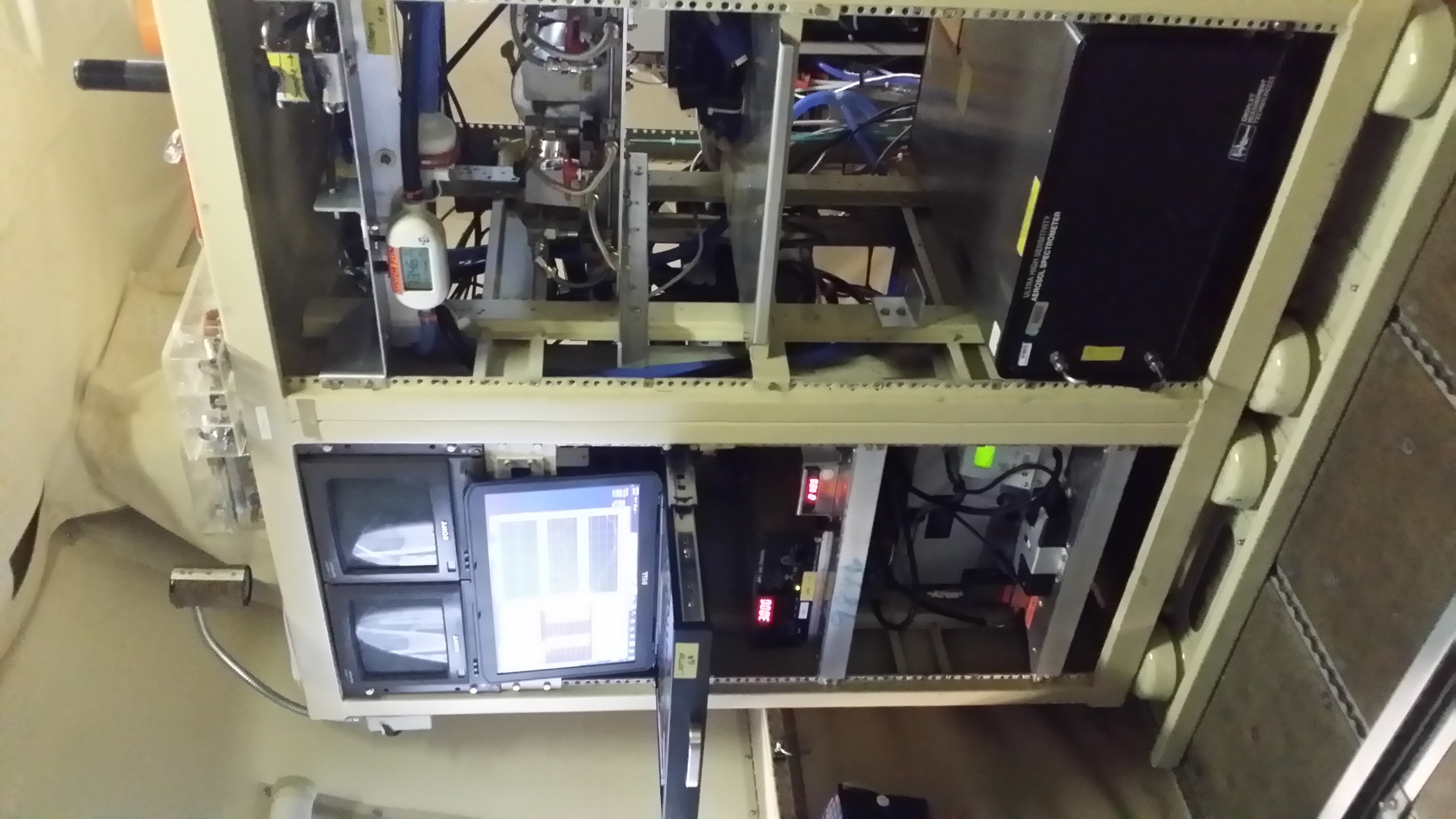
Front-view of the LARGE rack onboard the NOAA WP-3D aircraft.
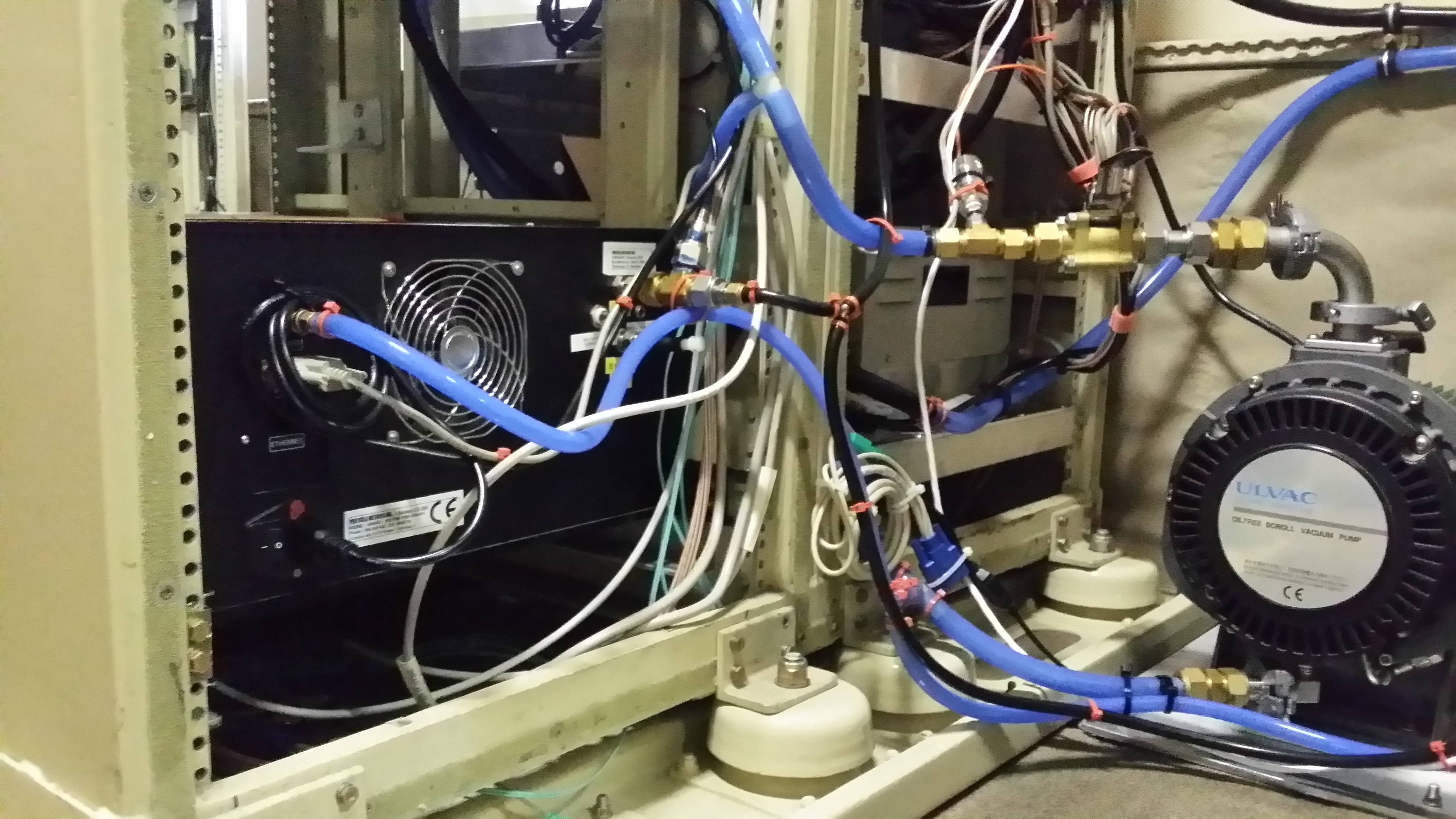
Back-view of LARGE plumbing.
We still have work to do to complete our instrument integration, especially to install an aerosol inlet on the aircraft. This will be completed soon and we will be poised to participate in the next hurricane flights! Check back later for more details about our instrumentation, science objectives, and pictures from inside the next Atlantic hurricane…
More information on our research can be found at the links below:
LARGE: http://science.larc.nasa.gov/large/
NOAA P-3 aircraft at the Aircraft Operations Center: http://www.aoc.noaa.gov/aircraft_lockheed.htm
My apologies for the gap between blog posts. My day job has been pretty busy. And even though the NASA folks have already arrived safely to Tahiti as of May 5, 2014, I thought it was fitting to have one last blog post. We have talked a lot about ocean biogeochemical sampling, ocean chemistry, and ocean color radiometry. It is also important to touch on the societal benefits that ocean color radiometry can provide.
In 2007, the International Ocean-Colour Coordinating Group or IOCCG published a report and an additional brochure entitled: “Why Ocean Colour? The Societal Benefits of Ocean-Colour Technology” and “Why Ocean Colour.” I will not go into all of the information detailed in each document here (though feel free to follow the links below at your leisure.)

IOCCG reports
A number of critical uses for ocean color are of particular importance in today’s society. For instance, detection of high algal biomass can indicate the location of potential fishing zone. Fish that eat algae or fish that eat fish that eat algae (did you get all of that?) will be en masse in these blooms. Inter-annual variation in timing and extent of phytoplankton blooms can also affect the survival of larval fish. Satellite imagery can be used to monitor this variation. Moreover, satellite derived sea surface temperature (SST) and wave height information can help aquaculture developers plan where to establish new fish farms. Satellite imagery can be used to detect and monitor blooms of harmful algae, algae (phytoplankton) that ether produce toxins or can clog the gills of fish and invertebrates because of high biomass.
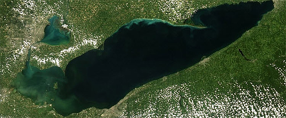
Harmful Algae Bloom in Lake Erie
http://oceanservice.noaa.gov/hazards/hab/
Satellite ocean color imagery is also very important for monitoring delicate ecosystems, particularly in global coastal environments. For example, the European Space Agency (ESA) has developed a program called CoastWatch that helps scientists harness the power of satellite imagery for monitoring water quality in shipping channels and coastal environments. The Medium Resolution Imaging Spectrometer (MERIS) on the Envisat platform (similar to NASA’s MODIS instruments) can be used to monitor sediment deposition onto coral reefs, which can smother the corals. The imagery can also be used to monitor water quality in shipping channels after dredging. Dredging can increase suspended sediments and negatively affect water quality.
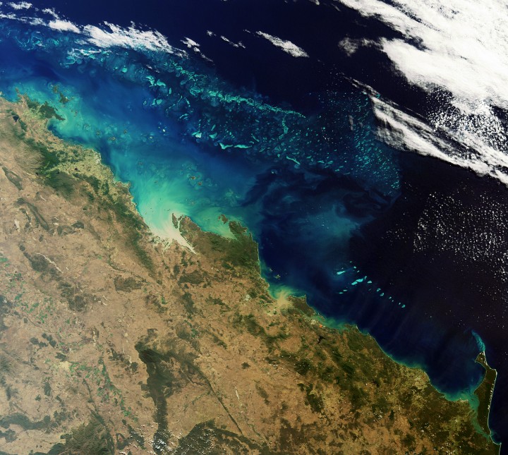
MERIS image: sediments flowing onto the Great Barrier reef in Australia
http://www.esa.int/Our_Activities/Observing_the_Earth/ESA_s_sharp_eyes_on_coastal_waters
Let’s consider a recent ecological disaster: the Deepwater Horizon oil spill. The Deepwater Horizon oil spill has been called the ‘worst oil spill in U.S. history’. The oil spill resulted from an oil platform explosion that occurred on April 20, 2010, and leaked an estimated 4.9 million barrels of oil by the time it was capped on July 15, 2010. This type of disaster can have long-term impacts on coastal wildlife and fisheries. Immediately following the spill, fishing areas around the Gulf Coast were closed to prevent human exposure to dangerous chemicals, polycyclic aromatic hydrocarbons, found in the oil. These chemicals are known to cause cancer. The fisheries were deemed safe and reopened on April 19, 2011.

Oil in the marshes of the Mississippi Delta
http://ocean.si.edu/gulf-oil-spill
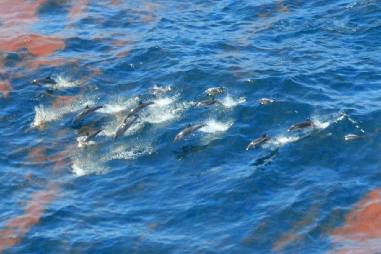
Dolphins swimming through the oil patches from the Deepwater Horizon spill
http://ocean.si.edu/gulf-oil-spill
Satellite ocean color imagery can be used to locate and monitor oil spills of this magnitude. Although this type of imagery is complex, the technology is a great asset. The video below, developed by video producers here at NASA Goddard, shows a timeline of NASA MODIS satellite images. Such imagery allowed scientists to follow the track of the oil slicks. These images can help us prepare for the impact of these disasters when we know where it is headed next. You can find satellite images of the oil spill here.
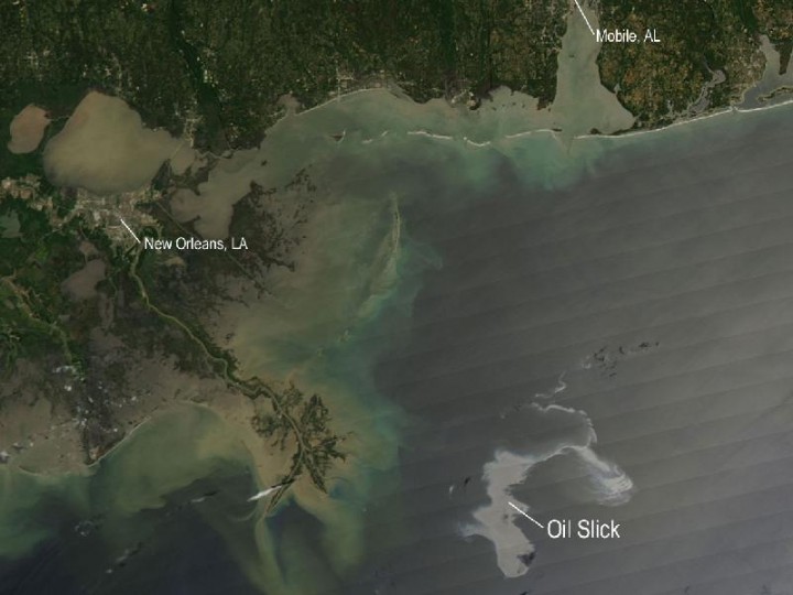
Satellite image of oil slick in the Gulf of Mexico following the sinking of the Deepwater Horizon platform
http://www.nasa.gov/multimedia/imagegallery/image_feature_1649.html
We have truly enjoyed sharing our experiences with all the blog readers. I hope we can do this again very soon. Until next time, make sure you check out all of the NASA field campaigns here at the Earth Observatory website.
http://www.ioccg.org/reports/report7.pdf
http://www.ioccg.org/reports/WOC_brochure.pdf
http://www.esa.int/Our_Activities/Observing_the_Earth/ESA_s_sharp_eyes_on_coastal_waters
http://www.esa.int/Our_Activities/Observing_the_Earth/New_ESA_project_supports_aquaculture
http://ocean.si.edu/gulf-oil-spill
http://www.nasa.gov/topics/earth/features/oil-spill-video.html
http://www.nasa.gov/topics/earth/features/oilspill/index.html
The global ocean is made up of five major ocean basins: the Pacific, Atlantic, Indian, Southern and Arctic Ocean. The Pacific Ocean is the largest of these basins as well as the deepest. Its expanse runs 155 million square miles and contains “more than half of the free water on earth.” Not only is it the largest and deepest ocean basin, but it is also the oldest, comprised of rocks that have been dated to be 200 million years old. You may have heard the term “Ring of Fire” associated with the Pacific Ocean. This name stems from the fact that the Pacific Ocean is prone to earthquakes and formation of submarine volcanoes along its extensive ridge and trench systems.
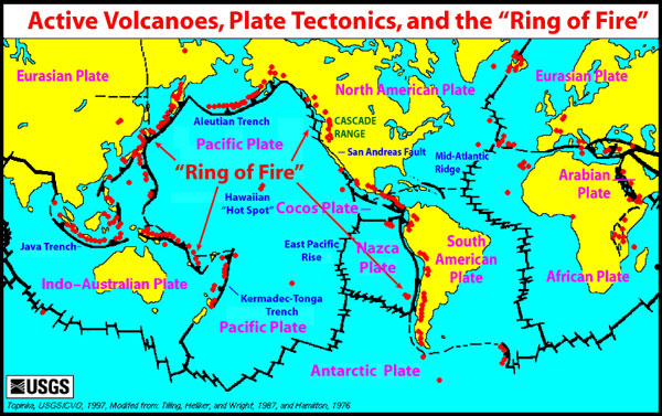
Ring of Fire
http://oceanexplorer.noaa.gov/explorations/05fire/background/volcanism/media/tectonics_world_map.html
The Pacific Ocean gained its name in the 16th century from the Portuguese navigator Ferdinand Magellan. Magellan and his crew set sail from Spain in 1519 in search of the Spice Islands located to the northeast of Indonesia. The Spice Islands were the largest producers in the world of spices such as nutmeg, cloves, and pepper. They navigated through the Atlantic Ocean and around the tip of South America after which they came across an unfamiliar ocean. He called this ocean ‘pacific’ which means peaceful. Unbeknownst to them, they still had a long journey to the Spice Islands. You can learn more about the voyage of Magellan and his crew here.
Magellan’s Voyage
http://news.bbc.co.uk/2/hi/science/nature/6170346.stm
OK, back to science! The CLIVAR P16S field campaign has entered the waters of the South Pacific known as a subtropical gyre. Gyre means “circular or spiral motion.” In the ocean, wind generated surface currents travel in a circular direction, either clockwise or counterclockwise, forming a large, circular body of water. The circular direction of the currents is caused by the Coriolis Force acting to deflect motion to the right in the Northern Hemisphere and to the left in the Southern Hemisphere due to the Earth’s rotation. The South Pacific gyre is located in the Southern Hemisphere, so winds and water are deflected to the left. Because of the deflection to the left, the gyre circulates in the counterclockwise direction, forcing water to pile up in the center of the gyre. In the last post, “An Appreciation for True-Color Satellite Imagery” we discussed how microscopic plants, or phytoplankton, require nutrients to grow. Blooms (large cell numbers) of phytoplankton cannot grow in these gyres because the water that piles up within the center of circulation is nutrient deficient.
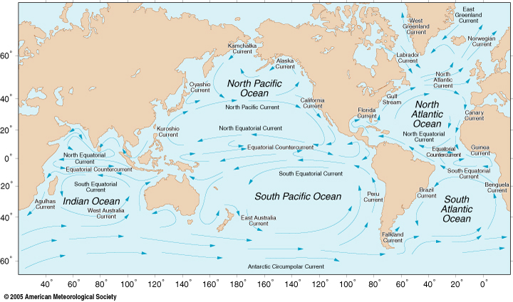
Global Ocean Circulation
http://oceanmotion.org/html/background/wind-driven-surface.htm
We can use the information about the color of the light being absorbed and reflected by the ocean to deduce the concentration of phytoplankton biomass using the proxy Chlorophyll a. Chlorophyll a is a pigment that both land plants and phytoplankton use to convert light to sugars in their chloroplast. Chlorophyll a absorbs strongly in the blue color of light. So when there is a lot of Chlorophyll a, then the light reflected back includes very little blue light. When there is very little or no Chlorophyll a, then a lot of blue light is reflected back. The figure below is an ocean color image based on the information I just described. The blue color represents little to no Chlorophyll a (or phytoplankton) present while the bright colors of yellow green and red represent increasing concentration of Chlorophyll a or phytoplankton biomass.
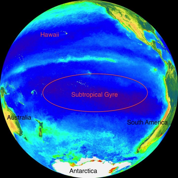
SeaWiFS Ocean Color image, Pacific Ocean
http://oceancolor.gsfc.nasa.gov/cgi/image_archive.cgi?c=CHLOROPHYLL
Please bear in mind that this explanation is very simplistic. You can learn more about how ocean color works here.
See the image below for the current cruise track of CLIVAR P16S. They are almost in Tahiti. Just a couple more weeks…
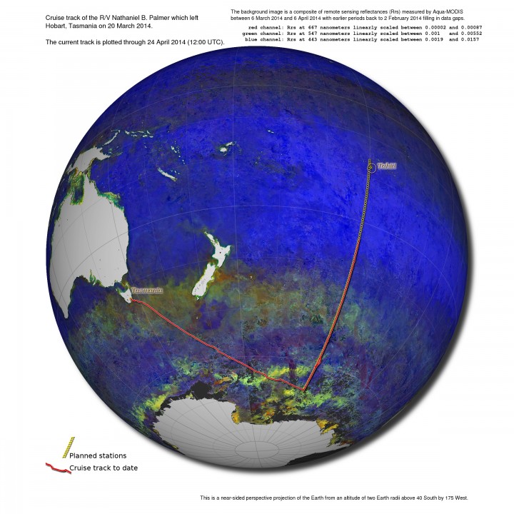
Cruise Track, CLIVAR-P16S
ACKNOWLEDGEMENTS: NASA’s Ocean Ecology Laboratory Field Support Group is participating in the US Repeat Hydrography, P16S field campaign under the auspices of the International Global Ocean Ship-Based Hydrographic Investigations Program (GO-SHIP). The US Climate Variability and Predictability Program (CLIVAR), NOAA and the NSF sponsor this campaign.

http://oceanservice.noaa.gov/facts/biggestocean.html
http://oceanservice.noaa.gov/facts/pacific.html
http://www.iol.ie/~spice/Indones.htm
http://www.rmg.co.uk/explore/sea-and-ships/facts/faqs/what-and-where-are-the-spice-islands
http://news.bbc.co.uk/2/hi/science/nature/6170346.stm
http://www.merriam-webster.com/dictionary/gyre
http://ww2010.atmos.uiuc.edu/(Gh)/guides/mtr/fw/crls.rxml
http://oceanworld.tamu.edu/students/currents/currents3.htm
http://oceancolor.gsfc.nasa.gov/cgi/image_archive.cgi?c=CHLOROPHYLL
http://oceancolor.gsfc.nasa.gov/SeaWiFS/
By Ludovic Brucker
After an unexpected phone call from the helicopter pilot on Easter Sunday, Ludo and Clem ended the second season of the Greenland aquifer campaign, with the support of Susan, Rick, Lora, Bear, the weather office, and many others. Thanks all for this Easter bunny.
We still wonder whether our campaign was successful, or fair. For sure, it was a mix of good and tough times.
The pluses, making our campaign a good time:
– We’re back from our field site, healthy and with all our fingers and toes!
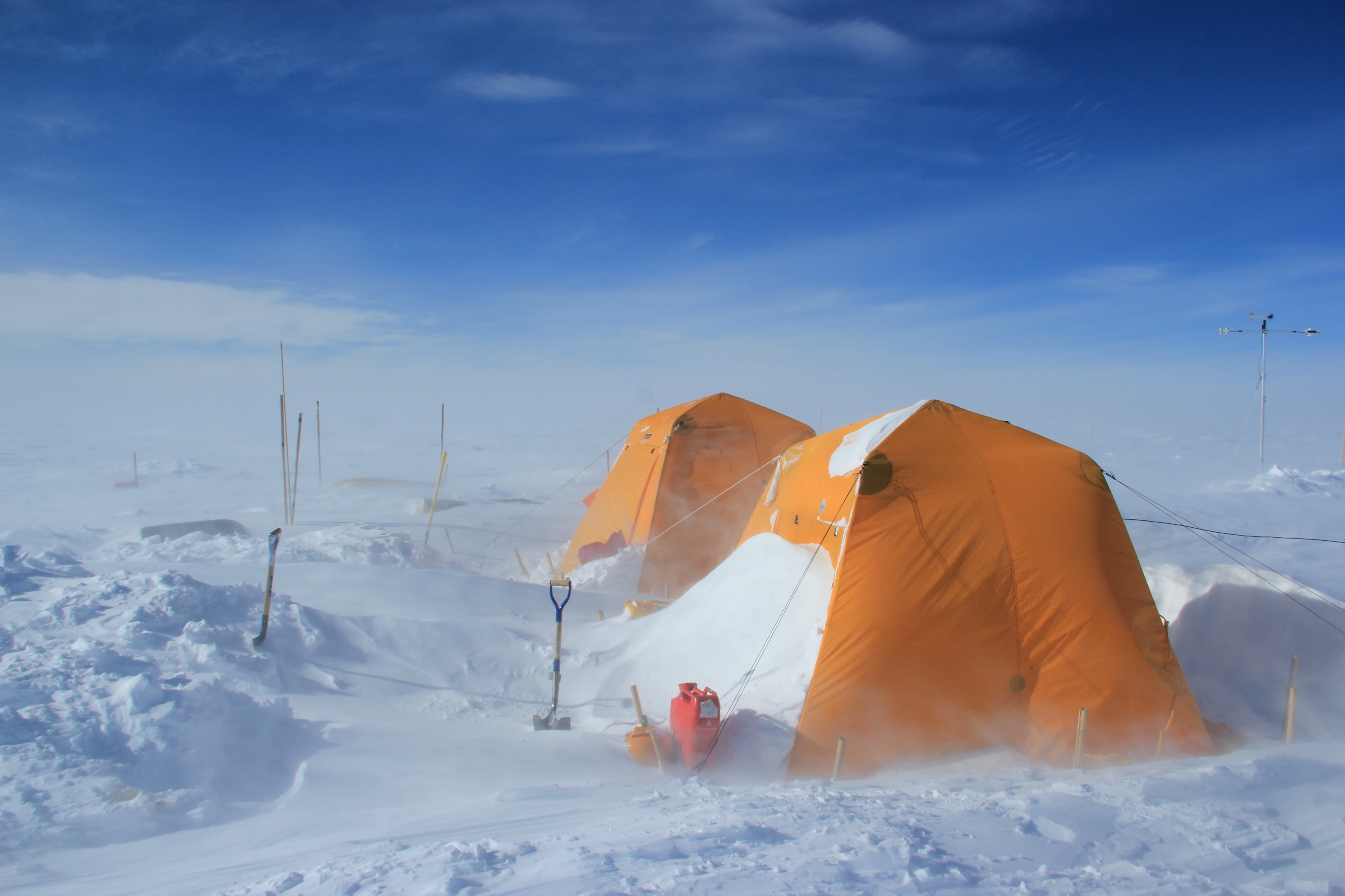
– We set up an almost perfect camp, limiting drift considerably.
– Our two tents survived 65-knot winds!
– We had saucisson (dry cured sausage), and cheese for fondue!
– No polar bear smelled our food!
– We collected over 17 miles (28 kilometers) of high-frequency (400 MHz) radar data, including 12 mi (20 km) in one day (equivalent to half a marathon!)
– Along a 1.24-mi (2-km) segment of the 2011 Arctic Circle Traverse, we deployed 5 radars operating at 400, 200, 40, 10, and 5 MHz.
– We installed an intelligent weather station developed by the group at IMAU, in the Netherlands.
– We drilled down to 28 feet (8.5 meters) to record the density and stratigraphy of the ice layers.
– We have GPS taken positions during a week, which will help us calculate the velocity and flow direction of the ice in this basin.
The minuses, making our campaign “different”:
– Ten days of weather delays before the put-in flight to our ice camp location.
– Rick could not make it to the field with us.
– We never had three consecutive half days with weather suitable for work.
– Getting a sore throat from shouting to hear each other less than a meter apart.
– During the one day of great weather, we tried to drive down a pilot tube to install a piezometer in the aquifer. This technique is adapted for ground water found within rocky soils. It was the first attempt to do it in the Greenland firn. Driving the metal pipes in the snow through the ice layers was a nightmare, we had to pound on those pipes really hard to make them go through the thick ice layers and we ended up breaking them. At one point, we thought it was broken slightly deeper than 6 ft below the surface, so we dug a pit down to fix it. Well, it turned out that the broken piece was actually 13 ft down — we spent the only full day of great weather breaking our equipment.
– We ran out of cheese for fondue, and of saucisson.
– Sunscreen was completely useless this season.
The “funny” stuff:
– 30 m/s wind is brutal, though not necessarily hilarious.
– High-wind speed does not make the clock spin faster, only the anemometer.
– Supporting text messages and jokes from our family, colleagues, and office mates.
– Attempting a radar survey with a sled taking off every other gusts.
– Calling the Met Office for a weather forecast: “Hello! Since it’s windy here we are wondering what will happen in the next 36 hours.” “Yes, I can confirm that you are experiencing wind.” “Thanks so much for the confirmation, but there was no room for doubt.” “Oh, but it’s a nice spike on the computer screen! It won’t blow more, but it won’t stop soon. Be careful out there”. Patience with Mother Nature is the #1 fundamental.
– Coastal storms from the East might be our favorite storms on the ice sheet: wind stops, and temperatures increase, but it snows, snows, and snows.
– Sixteen feet of seasonal snow is deep, especially with the top 2 feet of fresh snow becoming harder and harder as they it gets compacted by the wind.
– Excavating 1765 cubic feet of snow between 8pm and 11:30pm (you got to use the weather window whenever you have it.)
– The frost all around our sleeping-bag head every morning.
– The 40 hours laying down in the sleeping bag.
– The melody of the wind on our tents and through the bamboo sticks we stuck around them.
– Using the sleeping bag to store hats, balaclavas, gloves, socks, boot insulation, contact lenses, tooth paste, sun screen (it was nice to dream about the day we would need it), batteries, head lamp, snacks, water bottles (ideally liquid and not spilling.)
– The pilot phone call at 8 am on Easter Sunday: “Good morning, happy Easter! Don’t go for a ski strip today, we will come pick you up in 3-4 hours!”
This was the synopsis of our 13-day adventure on the ice sheet. Even though we have been pulled out from the ice sheet, we still have some work to do, such as cleaning and drying our cargo and repackaging it for shipping to either Kanger, or the US.
Now, we would like you to enjoy some photos taken in the field. Thanks again for spending some times reading the blog and following us! Until the next campaign, enjoy each season and stay warm! As we say in French: “En Mai, fait ce qu’il te plaît!” In English, it translates to something like: “In May, do as you please!”. Yup, we’re heading back to the office and will hide behind a computer screen for the months to come.
All the best,
Ludo & Clem
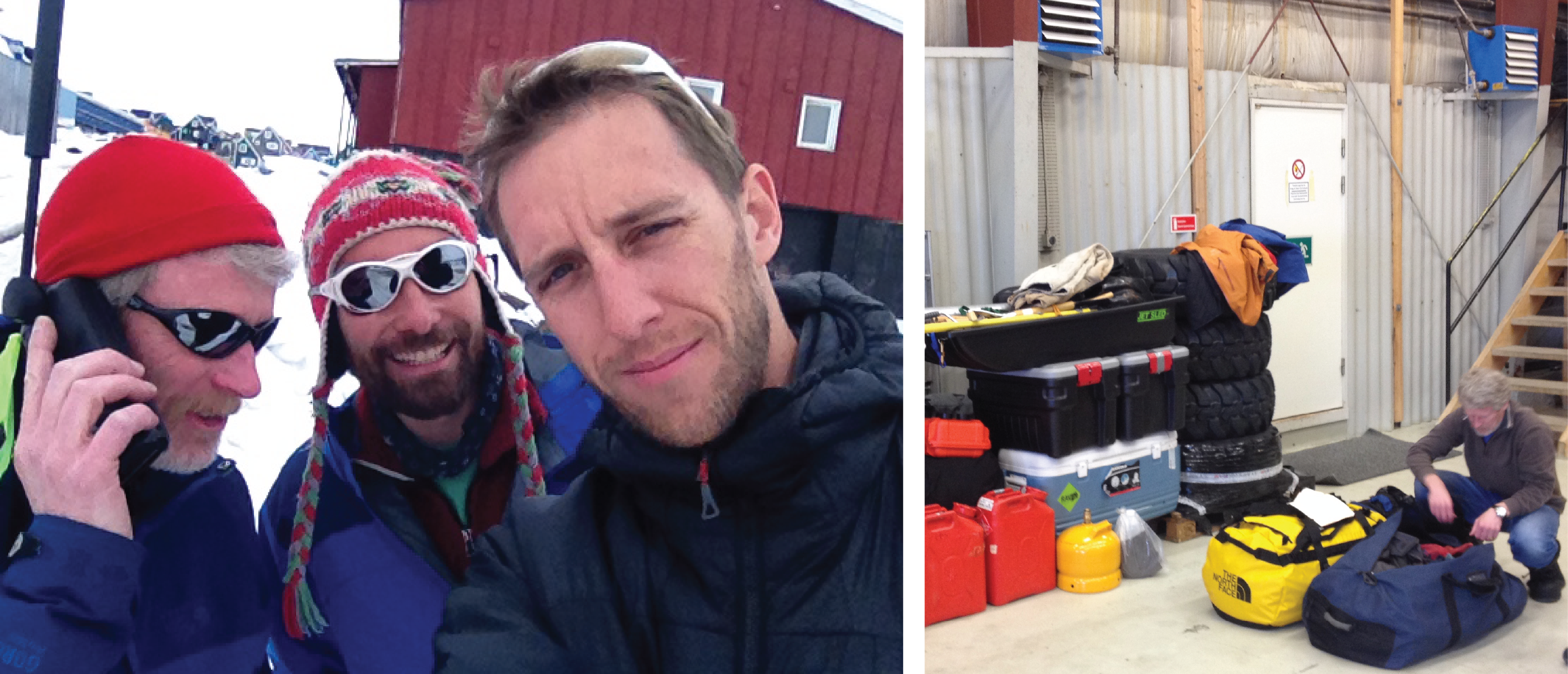
(Left) As weather-delay days continue to keep us in town, Rick calls the weather office to assess whether we can afford to spend more days waiting to be deployed on the ice sheet. (Right) The saddest moment of our campaign, when Rick had to remove his gear from our cargo because he wasn’t coming with us to the field.

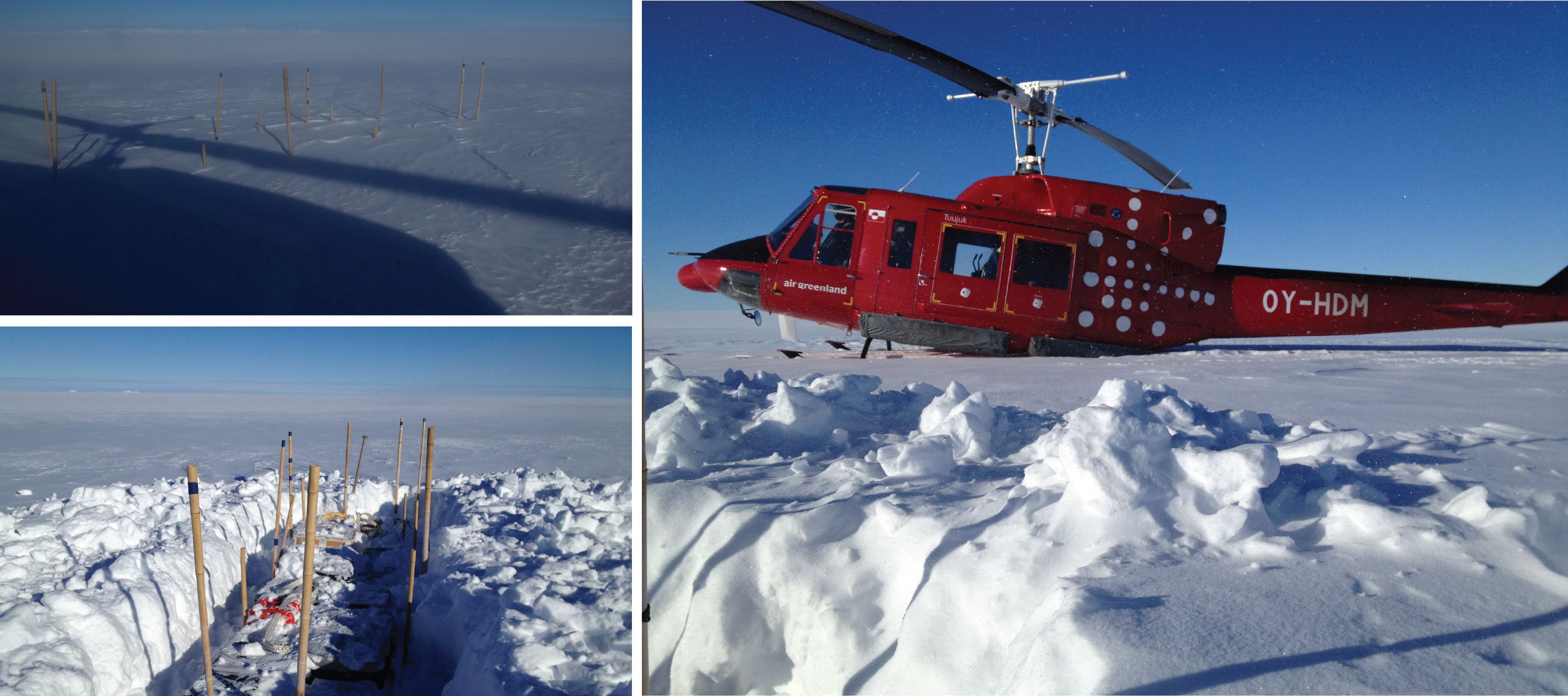
(Left) At the Tasiilaq heliport, Ludo waits for our put-in flight on the cargo. (Right) The Air Greenland B-212 helicopter with blue skies and high clouds. After 12 days of patiently waiting, it looks like it’s a go!
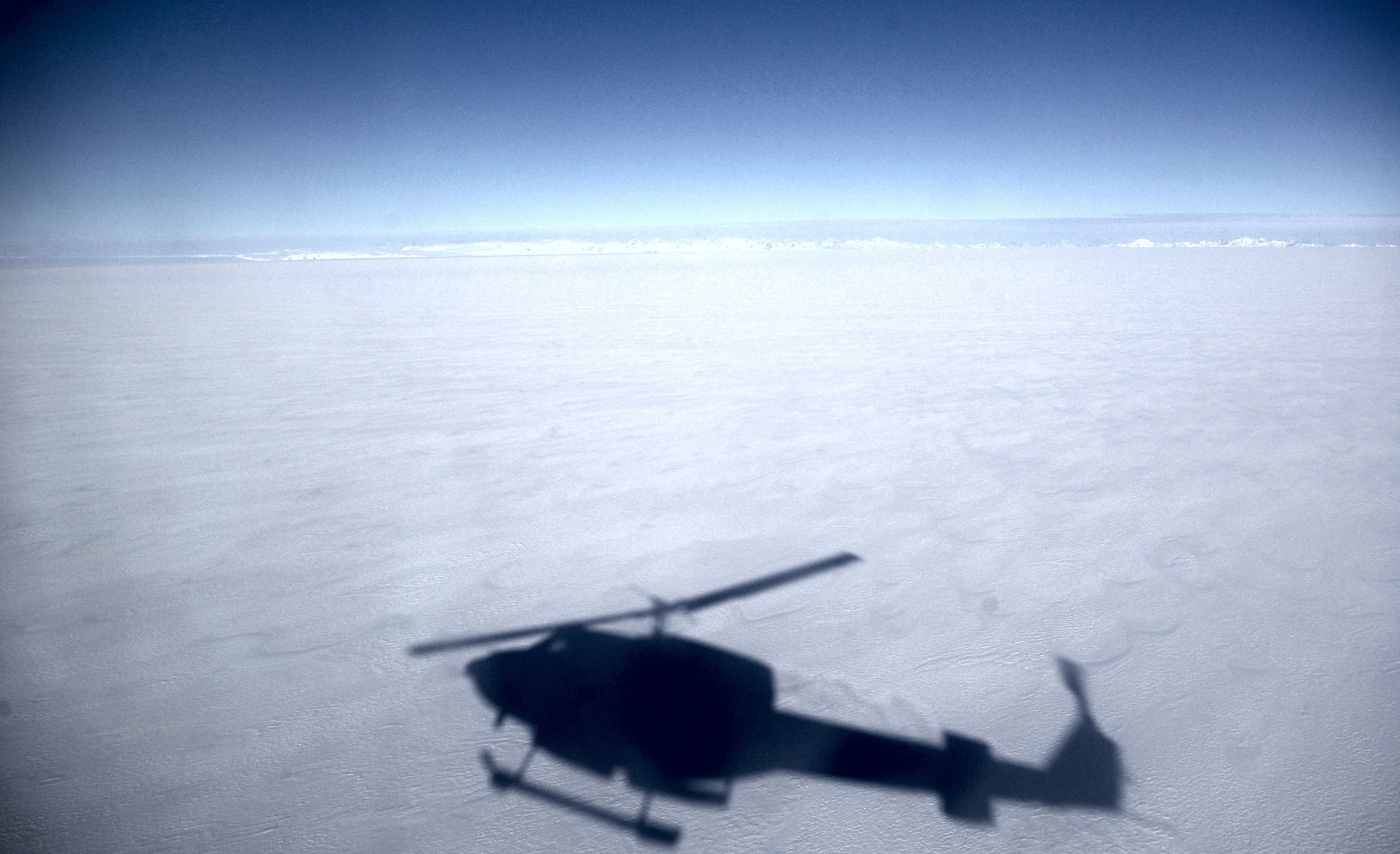
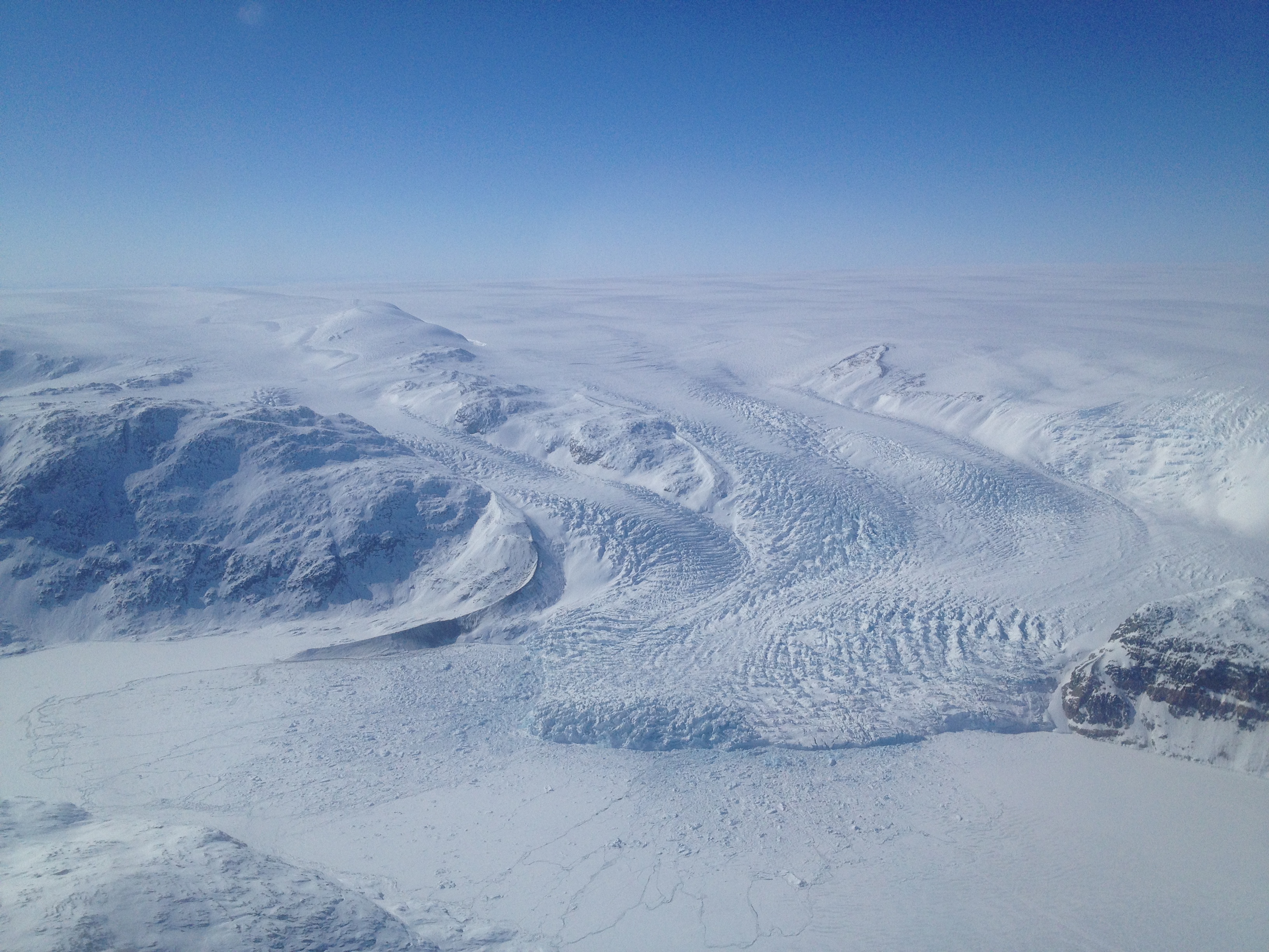
Flying over the sea-ice covered Sermilik fjord to reach the ice sheet.

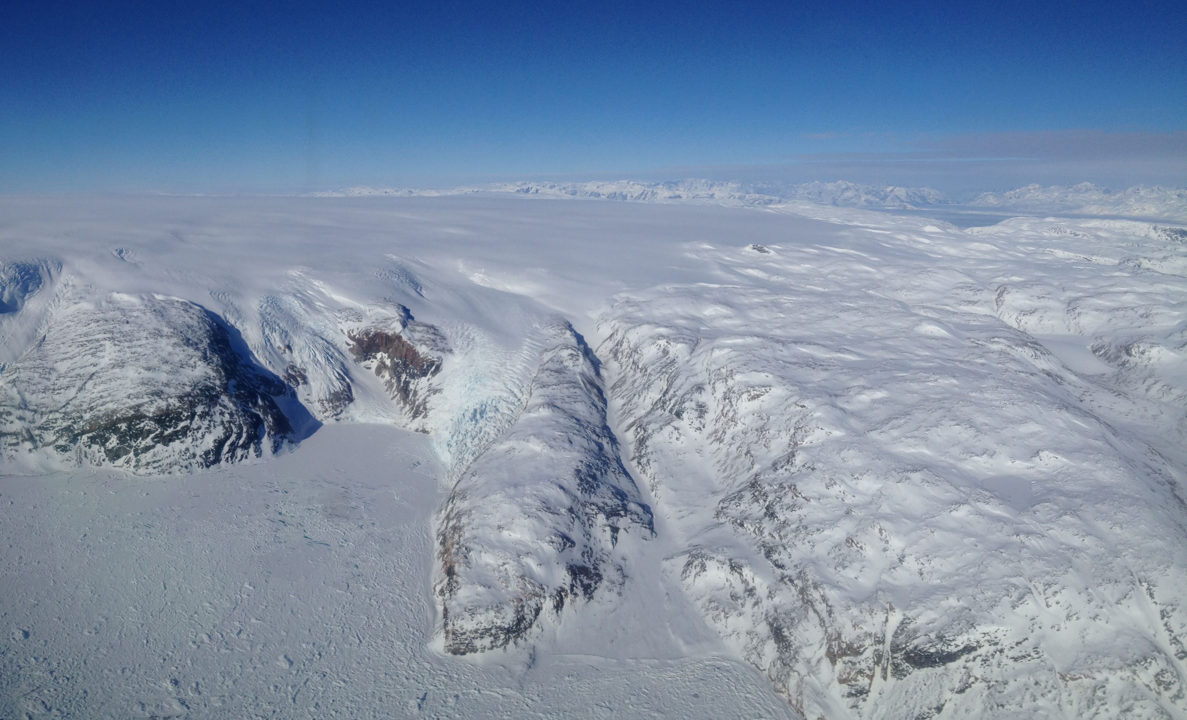
Getting closer to the ice sheet, flying over crevassed tributary glaciers.
(Left) Our cargo, dropped almost two weeks ago, got buried under 2 feet of snow. But all the pieces were there! (Right) The B-212 landed near our cargo for a final move to the ice camp location.
Approaching our camp site.
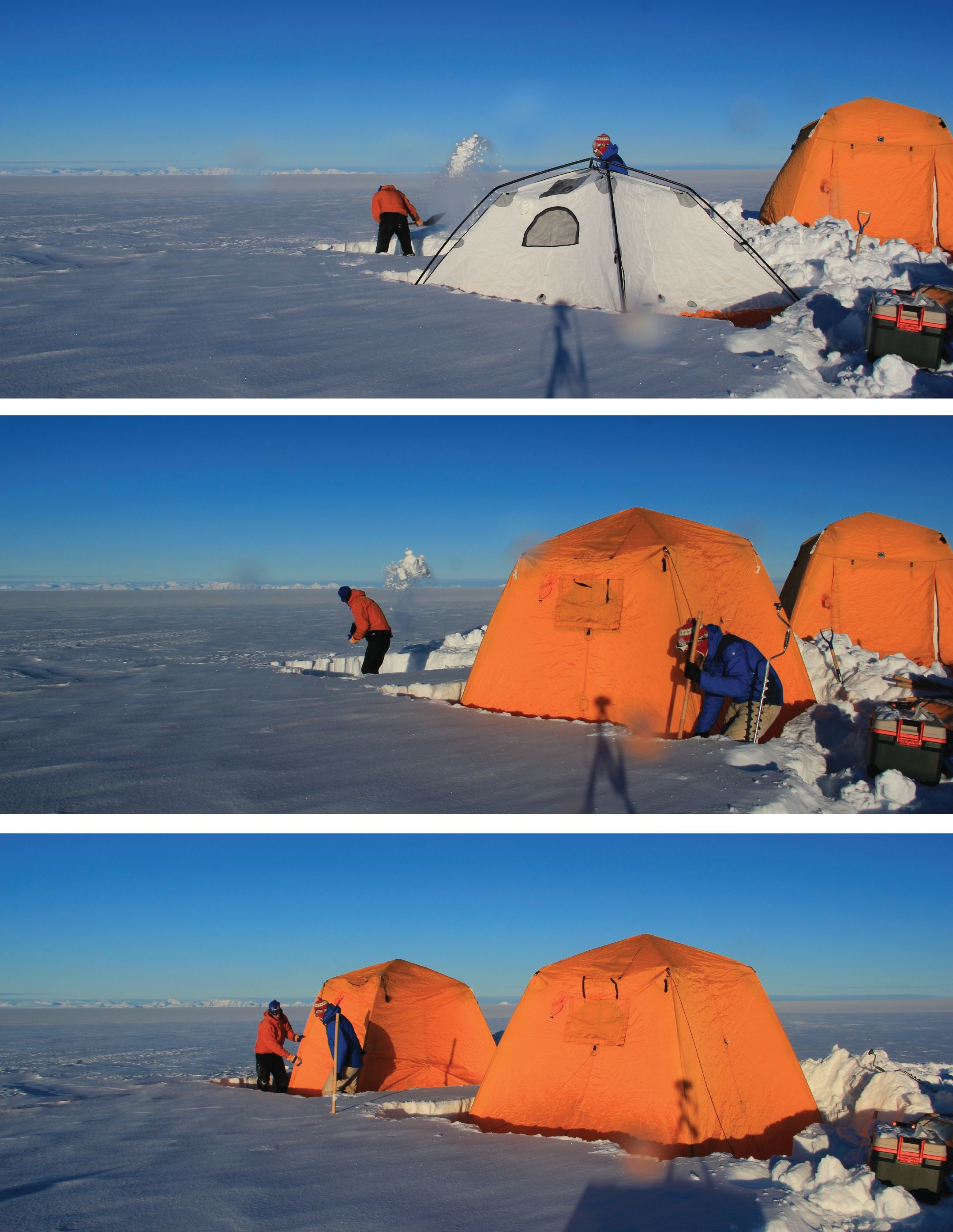
Minutes after the B-212 had left Clem and me on the ice sheet, we were already shoveling the fresh snow to install our cooking and sleeping tents before dark. This was no time for play, this was no time for fun, there was work to be done.
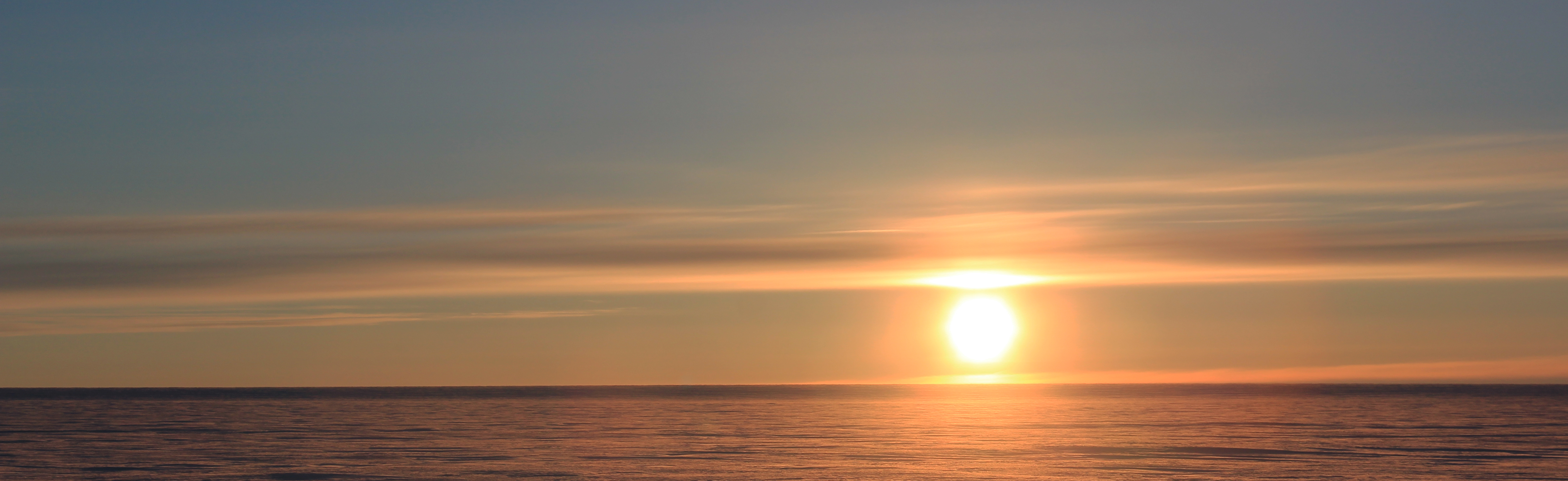
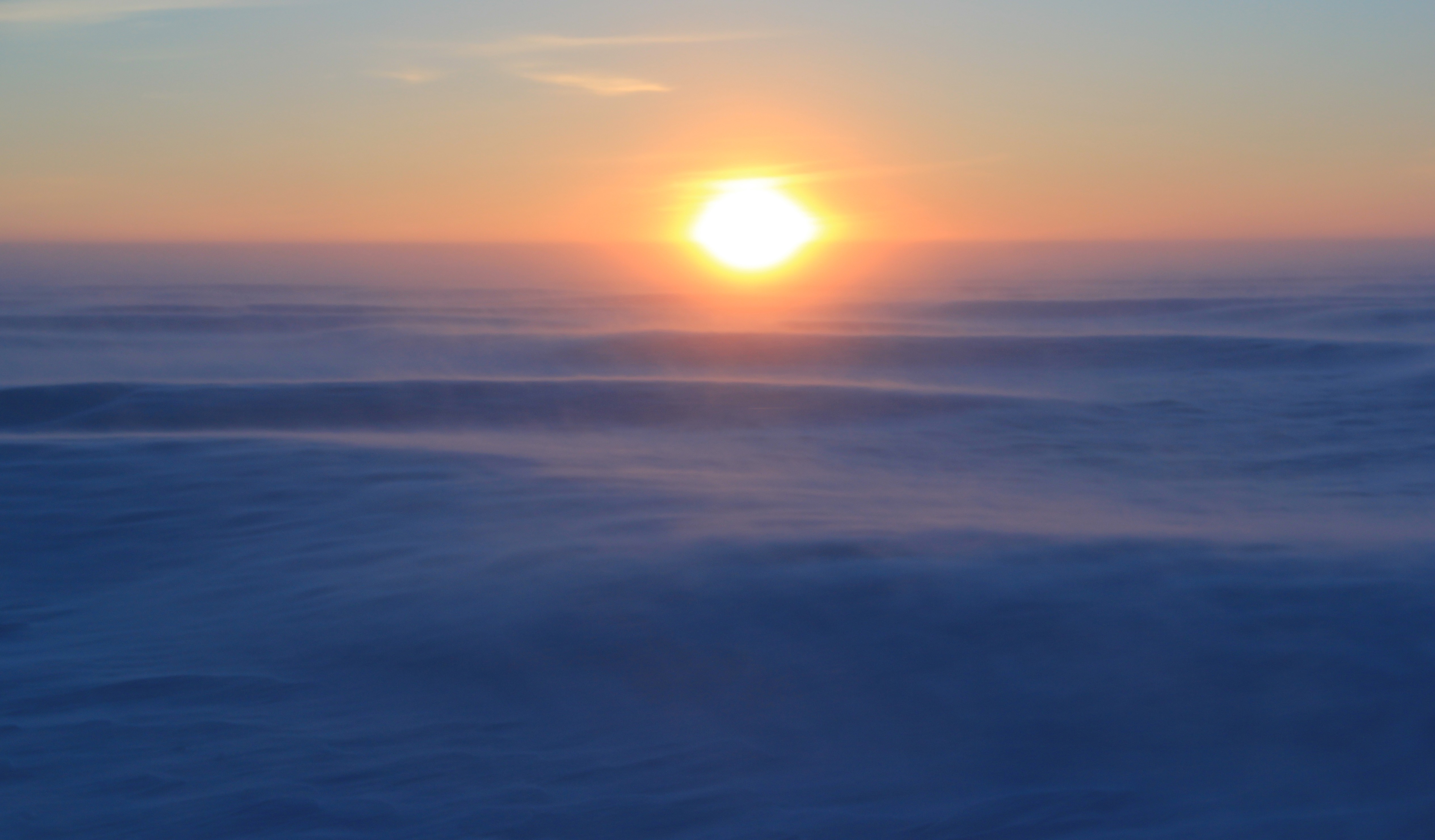
Our first pretty sunset in Greenland. In one month, we saw two of them.

Early morning selfie! Not fully ready yet to put our cold weather gear on.
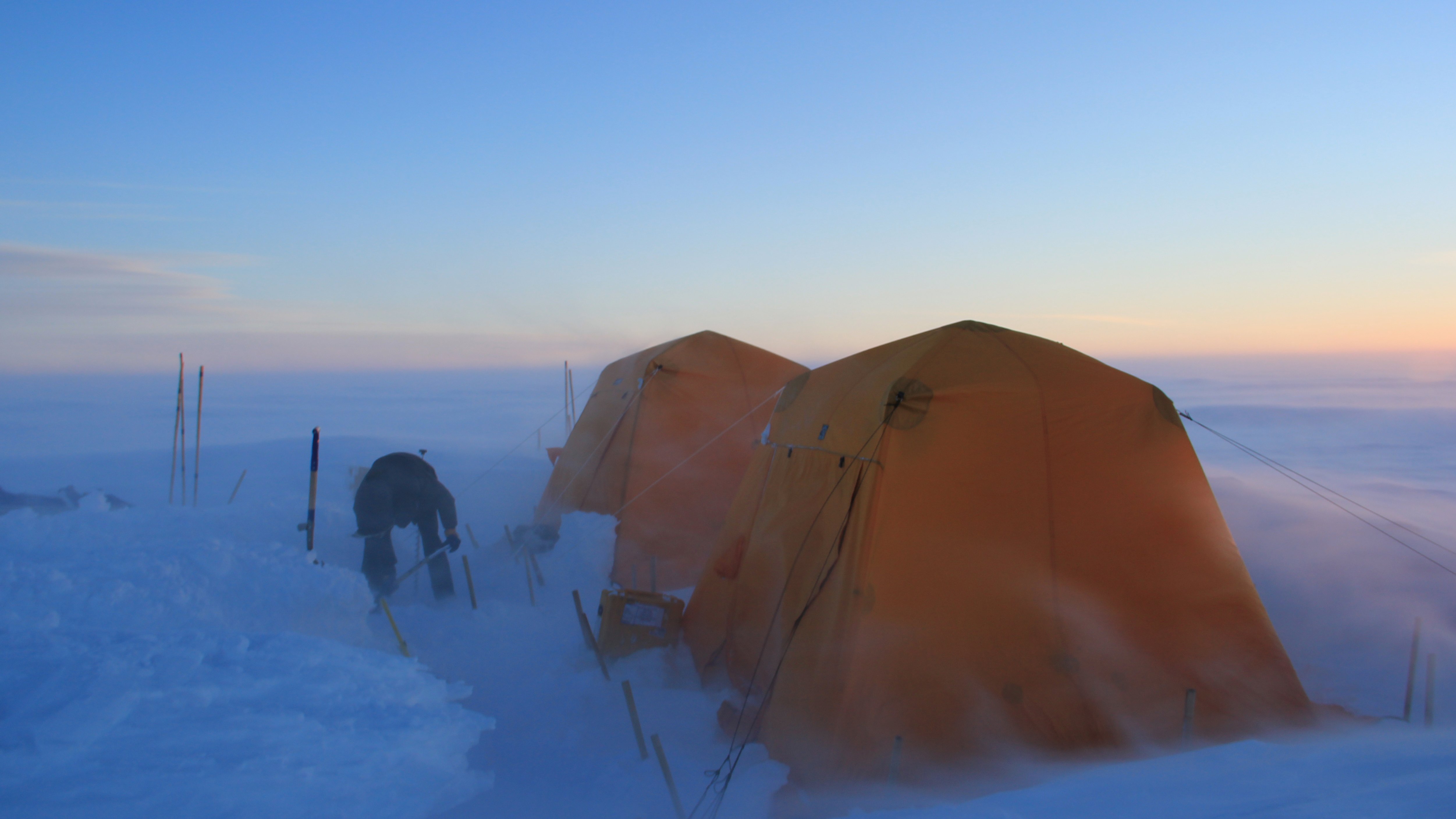
Shoveling, a typical activity at camp. Luckily this year we did not have to shovel too much to maintain our tents.
With the amount of fresh snow and the katabatic winds increasing, snow dunes were forming perpendicular to the direction of the wind — it was like being at sea! Half a day later, sastrugis developed along the wind direction and snow became hard and compact.
A snow drift blocking the door of the kitchen tent.
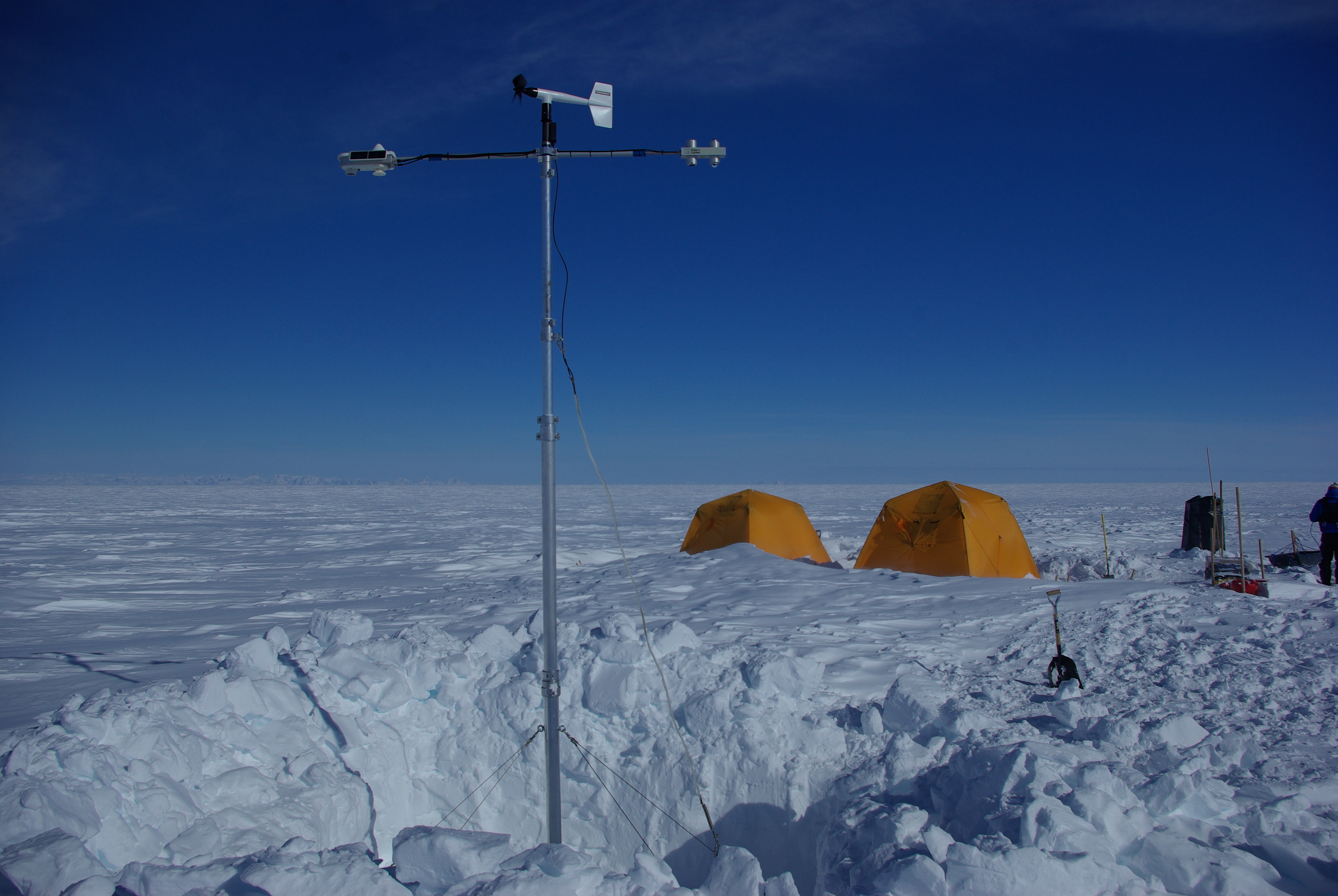
The IMAU intelligent Weather Station, installed in its snow pit before we refilled it.
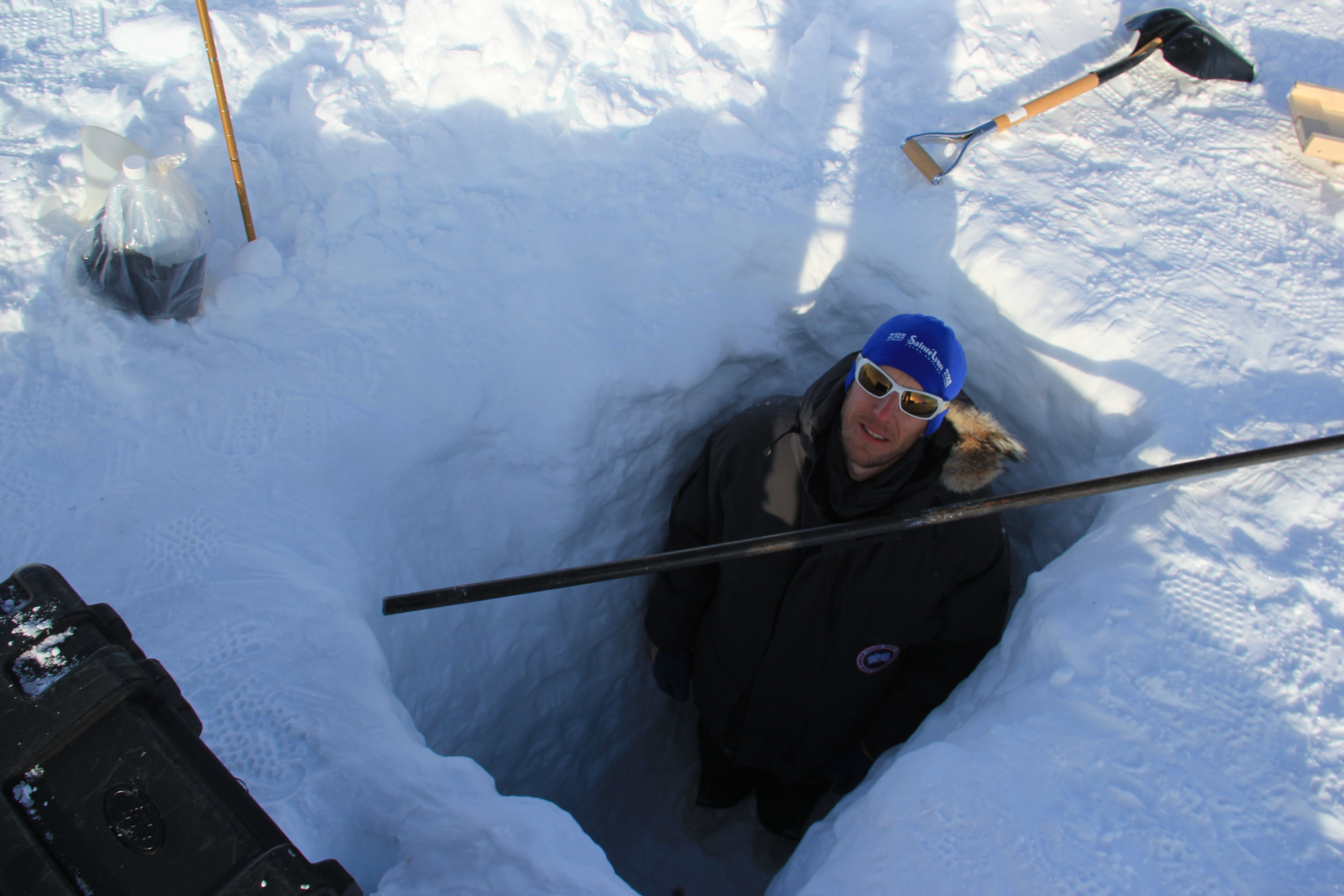
Ludo inside a 2-m-deep pit dug with the hope to repair a broken pilot pipe for installing a pressure transducer in the aquifer.
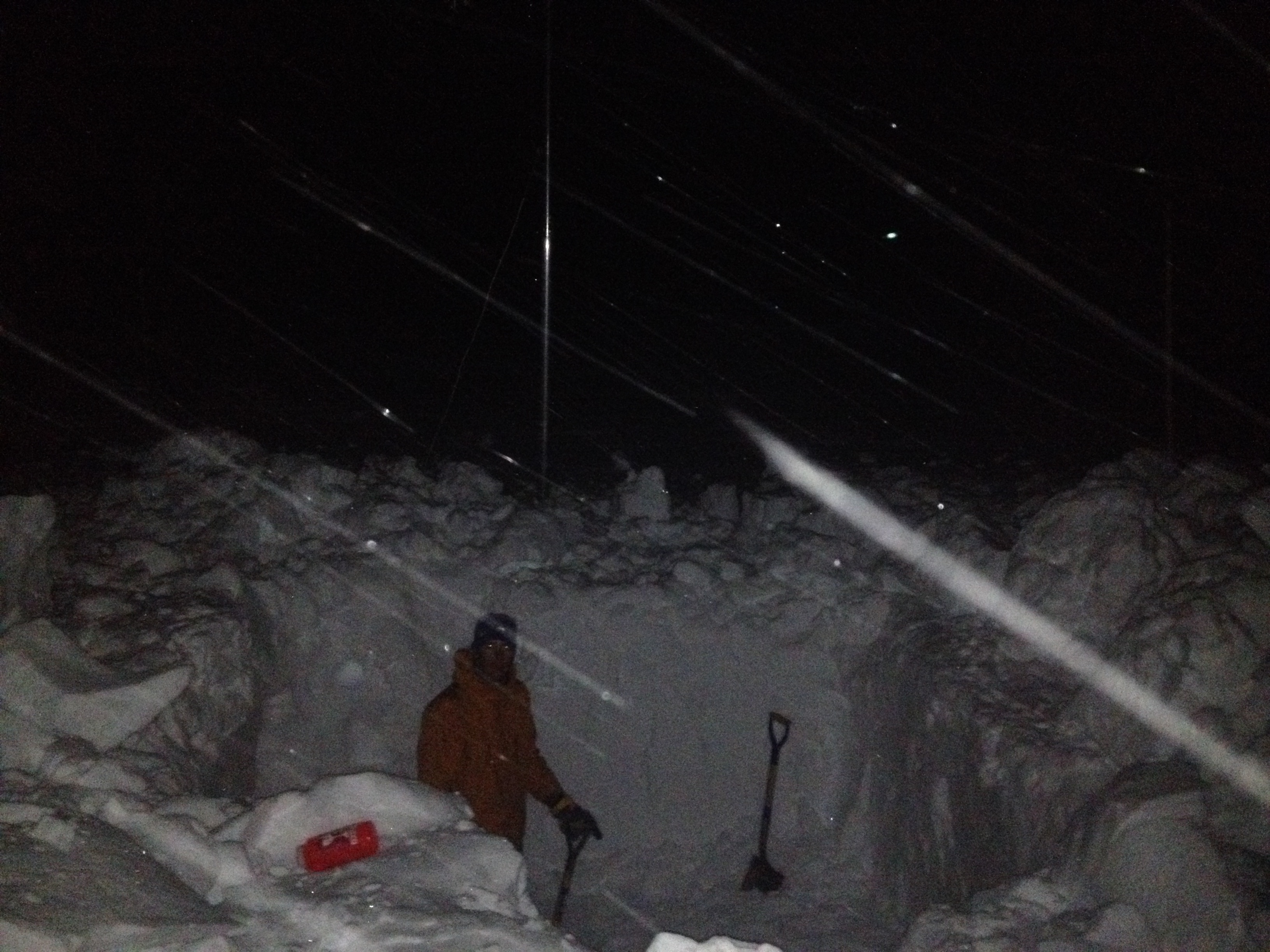
Ludo, inside a larger 2-meter-deep pit dug after dinner with easterly winds increasing as another coastal storm was coming bringing more snow. Our rationale was that the sooner we dug, the less snow we’d have to remove.

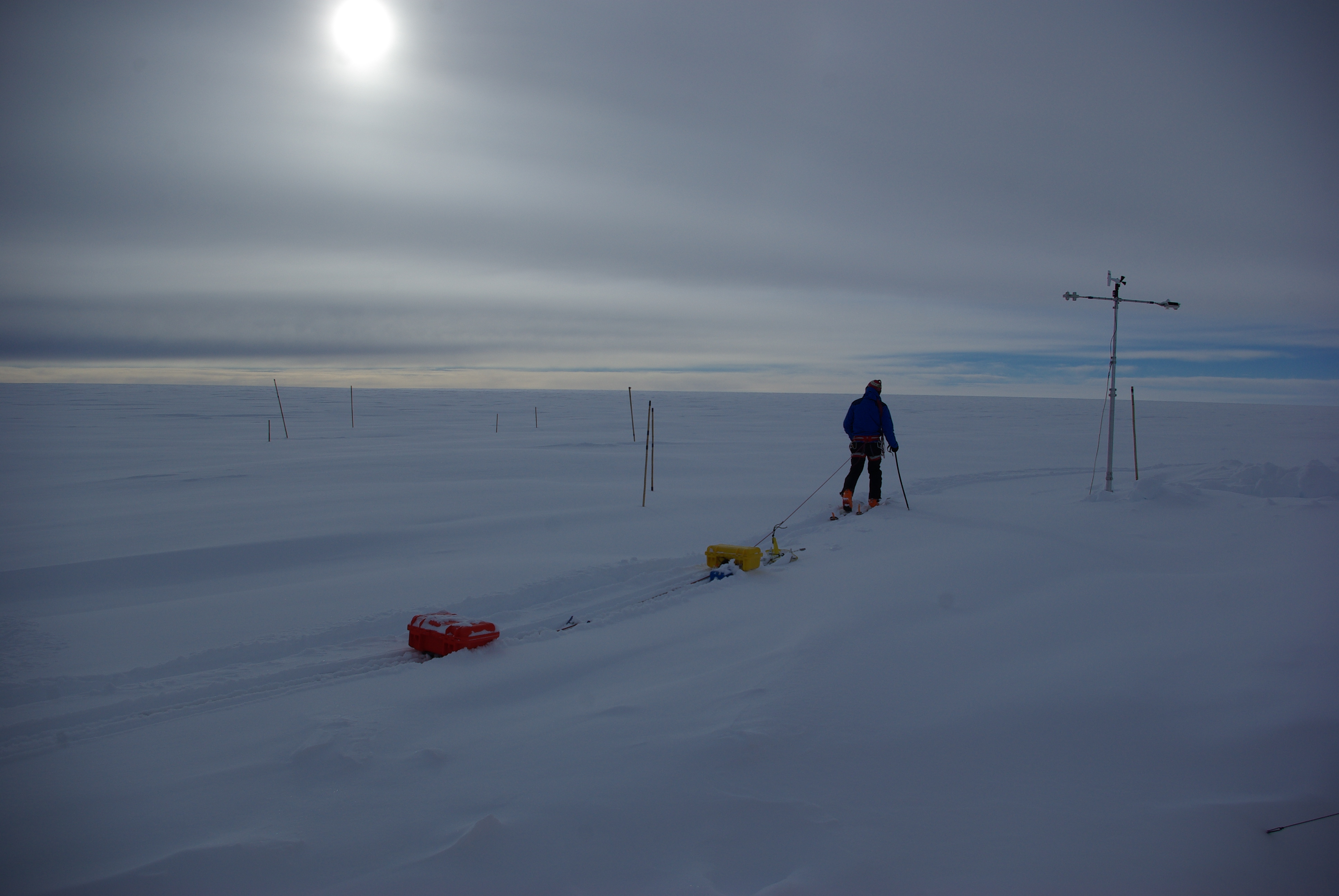
Two hours before being pulled out from the field, Clem was dragging the 200 MHz radar, and carrying a GPS unit.

(Left) Snow accumulated on our tent entrance overnight. We monitored it carefully every half hours from 2 am to the late evening. We took care of it a couple of times! (Middle) Clem calling the weather service to find out what wind speeds would hit us during the night. (Right) Our last saucisson, hanging over the snow/water pot.
Clem uses an evening break in the weather to drag a low-frequency radar in the fresh snow deposited in the previous hours.
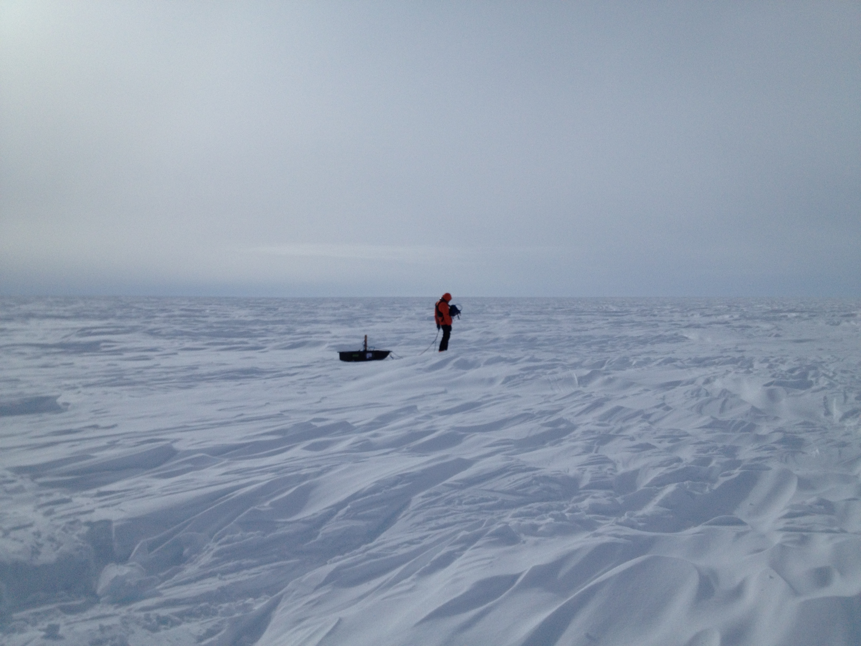
Clem dragging the 400 MHz radar over the sastrugis, a challenging surface to work with.
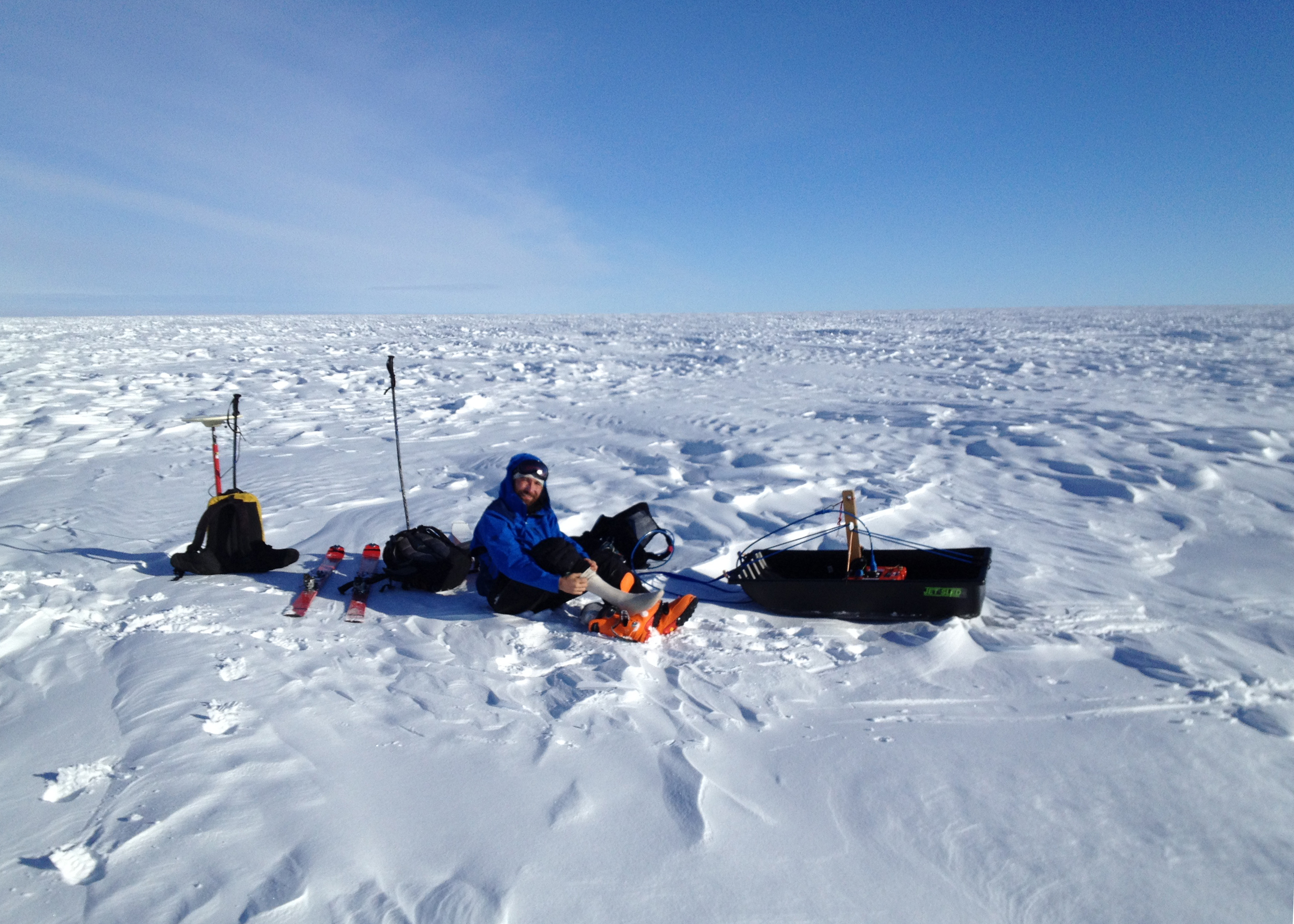
Weather was clement enough with Clément to allow him for a pit stop during our half-marathon radar day around camp.

A new day, different weather, and another attempt to collect more radar data. Since we aimed at collecting surface-based radar data, not airborne radar data, we quickly had to stop because the wind would make the radar system take off with every other gust.

Pictures taken just one hour apart. In the top one, we were setting up a radar system. In the bottom one, we were actively wrapping it due to sudden katabatic winds that picked up in less than 10 minutes.
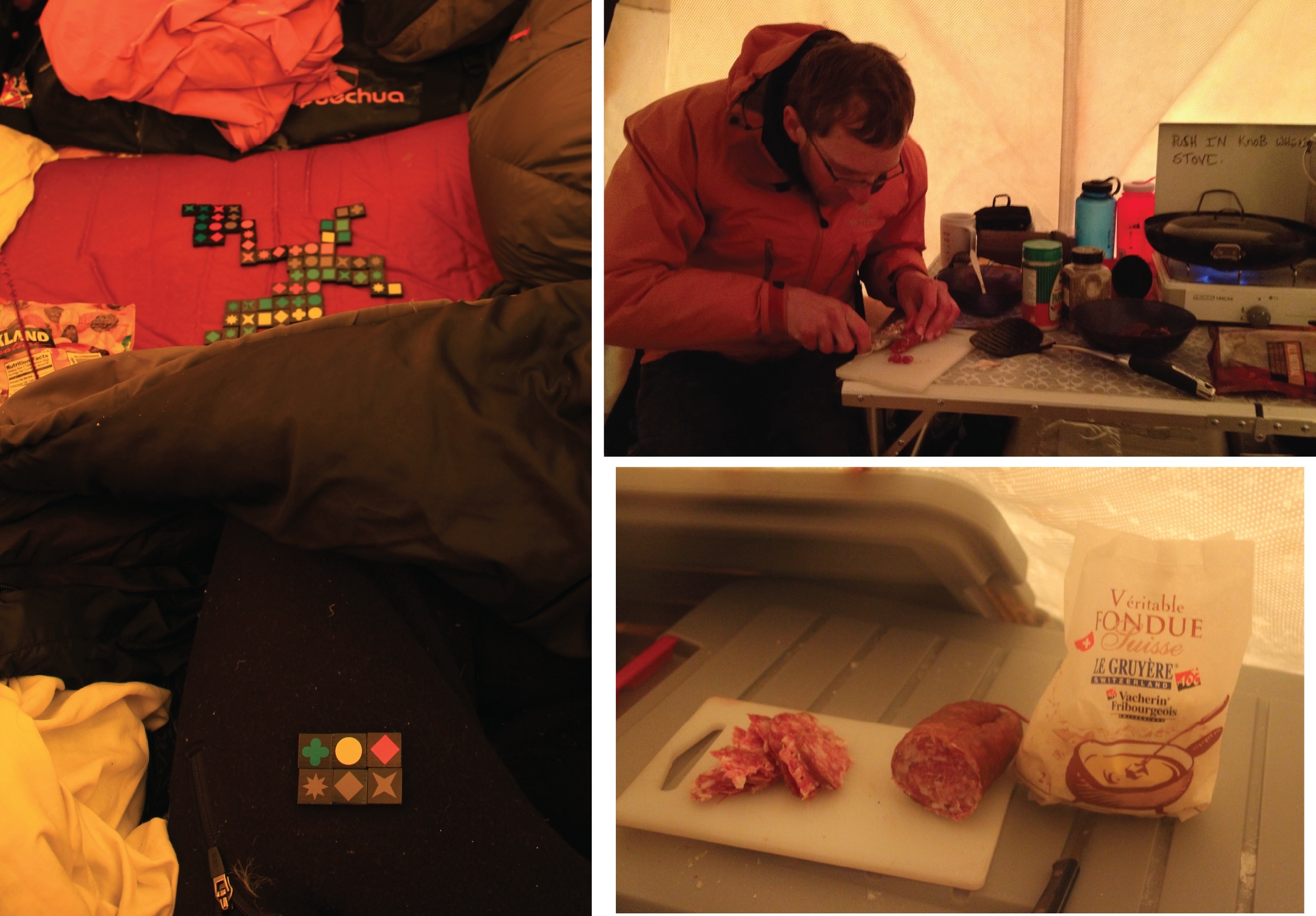
Indoor activities while the winds prevented us from working. (Left) Playing domino with mitts in a shaking tent, unforgettable times! (Right) Good food to keep us happy. Merci maman for thinking about us before leaving home.

Our flight back had already been canceled twice. It turned out that this was our last evening at camp. We had a total of two pretty sunsets: one on the first day and the second 12 days later, on our last evening.

Our bags, ready for a surprise pull-out flight! Happy Easter!

A great moment: the landing of the B-212. We were being pulled out!

The crew and Ludo finish up loading the B-212.
Last view of the ice sheet and glaciers.

Forty minutes after leaving our camp, we see signs of life: a view of Tasiilaq (top) and Kulusuk (bottom), minutes before landing.
We’d like to finish with this quote from the French explorer Jean-Baptiste Charcot, who led the second French expedition in Antarctica around 1910:
“D’où vient l’étrange attirance de ces régions polaires, si puissantes, si tenaces, qu’après en être revenu ou oublie les fatigues, morales et physiques, pour ne songer qu’à retourner vers elles? D’où vient le charme inouï de ces contrées pourtant désertes et terrifiantes?” (“Where does the strange attraction of the polar regions come from, so powerful, so stubborn, that after returning from them we forget the fatigue, moral and physical, only to think of returning there? Where does the incredible charm of these lands come from, however deserted and terrifying?”) Jean-Baptiste Charcot, Le Pourquoi Pas?
alert message
