Color the Bay Green (for Chlorophyll)

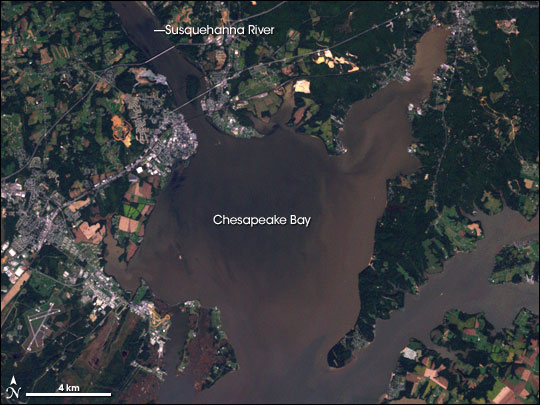
One of the scientists who examined the paper was Larry Harding of the Horn Point Laboratory of the University of Maryland Center for Environmental Science. Harding has studied the Bay for many years, and he has used remote-sensing data from satellite and aircraft-mounted instruments to investigate the biological behavior of phytoplankton in the Bay.

“Before I talked to Larry,” says Acker, “I wasn’t really aware that the upper and lower parts of the Bay were like two separate systems in many ways. I figured that the relationship between increased nitrogen and plant productivity applied to the whole Bay. I learned from Larry that that wasn’t the case.”

Harding explained that the largest input of nitrogen to the Bay comes from the Susquehanna River, which enters the northern reaches of the Bay at Havre de Grace after flowing through the fertile agricultural regions of Pennsylvania. There is so much nitrogen in the Susquehanna, even when drought reduces streamflow, that the growth of phytoplankton in the upper Bay is not limited by the availability of nitrogen. In other words, drought or no, the upper part of the Bay is probably going to bloom.

Only in the mid- to lower Bay, seaward of the large river outlets, is the growth of phytoplankton limited by nitrogen concentrations. In these regions, nitrogen availability varies greatly depending on freshwater flowing in from rivers and streams. When heavy rains—such as those in 2003—increase freshwater and nitrogen flow in the Chesapeake watershed, phytoplankton bloom in the mid- to lower Bay. When rainfall is less, nitrogen levels are lower, and phytoplankton growth is restricted. Under these conditions, Harding has reasoned, the lower Bay acts more like the coastal Atlantic Ocean.

When Acker’s colleague Suhung Shen correlated the freshwater flow data and monthly chlorophyll at the mouth of the Bay for 2002 and 2003, the researchers discovered that there was no correlation between flow rates and chlorophyll in 2002. In 2003, however, the team discovered a significant correlation between the rate of freshwater runoff and the chlorophyll concentration “downstream” at the mouth of the Bay – about one month later.

This observation made perfect sense. It would take a few weeks for the phytoplankton at the Bay mouth to respond to water with increased nitrogen concentrations flowing in from the upper Bay. And when very little freshwater flowed in, as in 2002, waters at the Bay mouth were “decoupled” from the Bay and behaved more like the waters of the coastal Atlantic Ocean. High flows of nitrogen-rich freshwater runoff appeared to reconnect the mouth of the Bay with the biological dynamics of the Bay itself.

Nitrogen in the Bay and Around the World

“This study provided more than I expected,” Acker said. “The observation of how freshwater flow influences phytoplankton at the mouth of the Bay is an indication that sufficient reductions in nitrogen entering the Bay will reduce the influence of the land, at least in the lower Bay. This study helps to confirm the important goal of nitrogen reduction in efforts to restore the Bay.”

The Susquehanna River, which enters the Chesapeake Bay at its northern end, carries 40 percent of the nitrogen that flows into the Bay—the largest single source. There is so much nitrogen in the northern Bay that algae have all the "fertilizer" they need, and changes in streamflow do little or nothing to affect the growth of algal blooms. This satellite image shows brown water flowing from the Susquehanna. (NASA image by Robert Simmon, based on Landsat-7 data provided by the UMD Global Land Cover Facility)

“We also learned how to better use Giovanni for research, and how it can be used with ocean color data to observe chlorophyll concentrations in coastal waters around the world that are not nearly as well studied as Chesapeake Bay,” he added. “There are vital estuaries in many countries that may have problems similar to those of the Chesapeake, and Giovanni could be used to monitor the impact of programs to reduce nitrogen pollution. Giovanni is so easy to use, it can allow many more marine scientists to enhance their current research and knowledge with ocean color data analyses.”

• Links:
• Giovanni: Ocean Color Time-Series Online Visualization and Analysis
• Creeping Dead Zones
• Chesapeake Bay Foundation
• USGS Water Resources of Maryland, Delaware, and DC Area
• EPA Chesapeake Bay Program Office

• References:
• Acker, J. G., L. W. Harding, G. Leptoukh, T. Zhu, and S. Shen, 2005: “Remotely-sensed chl a at the Chesapeake Bay mouth is correlated with annual freshwater flow to Chesapeake Bay” Geophysical Research Letters, 32.
• Harding, L. W., Jr., 1994: “Long-term trends in the distribution of phytoplankton in Chesapeake Bay: Roles of light, nutrients, and streamflow,“ Marine Ecology Progress Series, 104, 267–291.
• Harding, L. W., Jr., and E. Perry, 1997: “Long-term increase of phytoplankton biomass in Chesapeake Bay,” Marine Ecology Progress Series, 157, 39–52.
• Harding, L. W., Jr., A. Magnuson, and M. E. Mallonee 2005: “SeaWiFS retrievals of chlorophyll in Chesapeake Bay and the Mid-Atlantic bight,” Estuarine Coastal and Shelf Science, 62, 75–94.
• Malone, T. C. 1992: Effects of water column processes on dissolved oxygen, nutrients, phytoplankton and zooplankton, in Oxygen Dynamics in Chesapeake Bay: A Synthesis of Research, edited by D. Smith, M. Leffler, and G. Mackiernan, pp. 61–112, Univ. of Maryland Sea Grant College, College Park, MD
• Officer, C. B., R. B. Biggs, J. L. Taft, L. E. Cronin, and M. A. Tyler, 1984: “Chesapeake Bay anoxia: Origin, development, and significance,” Science, 223, 22–27.

Acknowledgment:
• Development of Giovanni for ocean color data analysis and research is supported by the Ocean Color Time-Series Project, NASA Research, Education and Application Solutions Network (REASoN) CAN 02-OES-01. Principal Investigator for the Ocean Color Time-Series Project is Watson Gregg, with Co-Investigators Wayne Esaias, Charles McClain, Gene Feldman, Steven Kempler, Gregory Leptoukh, and James Acker.

 Color the Bay Green (for Chlorophyll)

Dead zones are present in estuaries all over the globe, particularly near densely populated or intensively farmed areas. Each red dot on this map indicates a body of water prone to oxygen depletion and the formation of a dead zone. (Map by Robert Simmon, based on data provided by Robert Diaz, Virginia Institute of Marine Science)