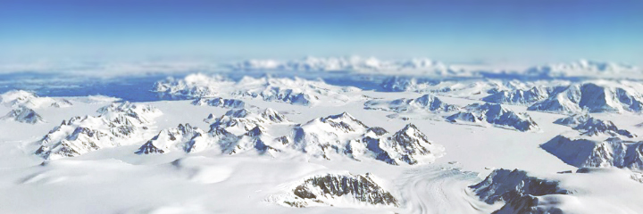
During a research flight on November 3, 2017, NASA scientist Nathan Kurtz snapped this photograph of glaciers east of Adelaide Island on the Antarctic Peninsula.
January 11, 2018
There’s something about Antarctica that attracts artists and photographers. The crowd near gate 14 at Jorge Newbery International Airport in Buenos Aires put it all in stark relief. Waterproof bags protected lenses large and small. A few people wore vests covered with pockets designed for the safe-keeping of lens caps and other gear. All of us were headed for Ushuaia, Argentina, which is frequently referred to as the southernmost city in the world and the gateway to Antarctica.
Most of those travelers were headed for cruise ships, from which they would photograph the icy continent. But I was not destined for a ship. On assignment for Earth Observatory, my vessel would be NASA’s P-3 research airplane. With camera and laptop in tow, I joined the aircraft crew and science instrument teams for several weeks as they made near-daily research flights.
The mission, called Operation IceBridge, is in its ninth year of flights to map the snow and ice of Antarctica. The view from above provides a tremendous amount of information about the huge expanses of snow and ice around Earth’s polar regions and how they are changing.
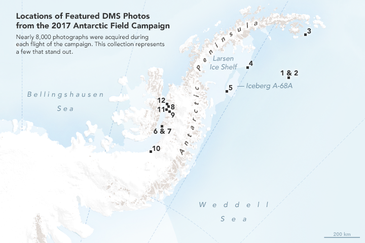
(NASA Earth Observatory map by Joshua Stevens.)
One of the mission’s instruments, the Digital Mapping System, collects thousands of high-resolution photographs during a single flight. These images shot from a camera mounted on the belly of the plane are “visual truth,” helping scientists identify features that are also detected by radar, laser, and gravity instruments.
The photographs below bridge the worlds of art and science. They were shot for research purposes, but there is no mistaking their beauty.
It takes a few hours to fly from the tip of South America to the parts of the frozen continent where scientists have been collecting data. Along most of the transit route, the Southern Ocean stretches as far as you can see. Depending on the winds, this expanse of gray-blue water can appear at times turbulent and at other times smooth (particularly in the vicinity of sea ice). Eventually flecks of icebergs begin to appear, followed by a thin layer of sea ice, and then the abrupt edge of an ice floe.
Some flight lines are designed to map the ice laying atop the land, while others map the sea ice. On November 4, 2017, the IceBridge team flew its “Endurance West” mission, which specifically targets sea ice. The P3 crossed the northern tip of the Antarctic Peninsula, descended to a lower altitude, and then flew southward across the Weddell Sea. The path purposely follows a ground track of ICESat-2 —an ice-mapping satellite mission that is scheduled for launch in late 2018.
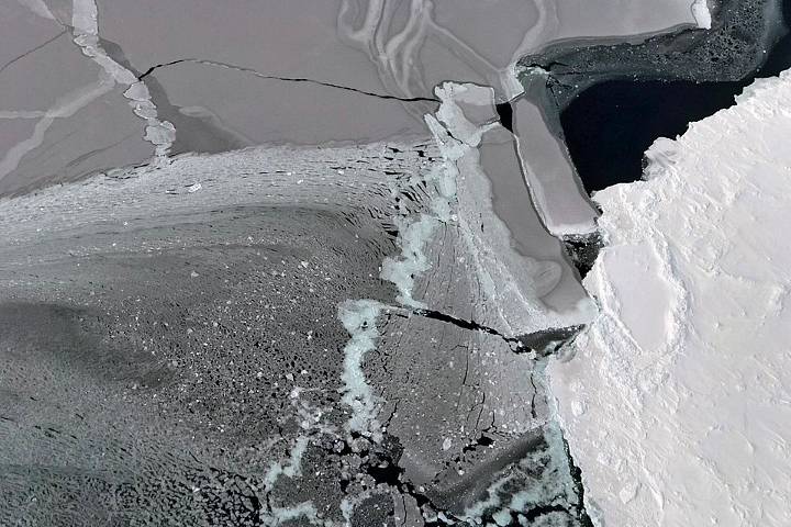
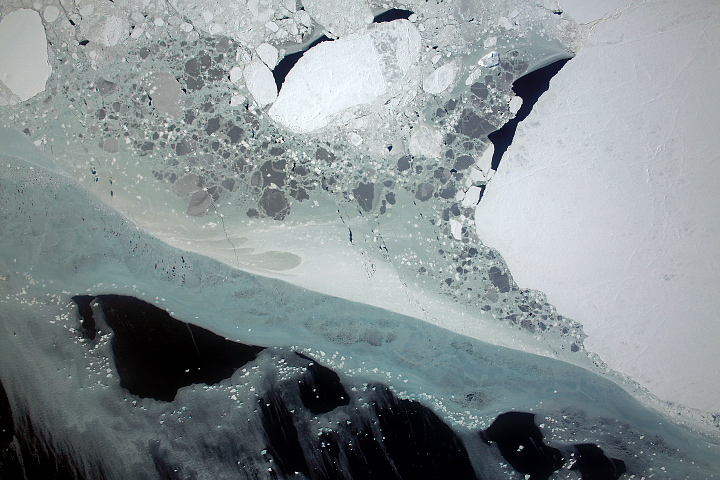
Images from that day show just how varied sea ice can appear. The first photograph, shot from the aircraft by IceBridge project scientist Nathan Kurtz, shows newly formed sea ice next to a snow-covered floe in the Weddell Sea. The second and third images, both acquired by the Digital Mapping System (DMS), show sea ice off the Antarctic Peninsula. Thicker ice is white, thinner ice is gray, and open water is black or navy.
1: Newly formed sea ice (gray) in the Weddell Sea. (Photo by NASA/Nathan Kurtz.)
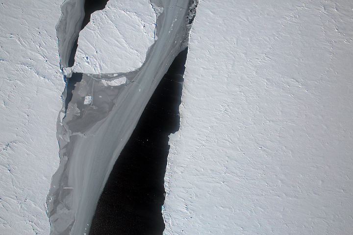
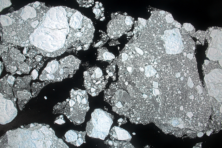
2: Thin ice fills the gap between two thicker ice floes. (Photo by NASA/Digital Mapping System.)
3: Pieces of sea ice, thick and thin, mingle in the Weddell Sea. (Photo by NASA/Digital Mapping System.)
On November 12, 2017, IceBridge flew a high-priority mission over the Larsen C Ice Shelf. In July 2017, this region was significantly reshaped by the shedding of an iceberg the size of Delaware. (You can read about what it was like to see that massive berg for the first time in this blog post, and you can see satellite images here.)
For most of the four-hour survey, as the aircraft flew back-and-forth in parallel lines over the ice shelf, the landscape appeared flat and white. These new flight lines followed the ground tracks of the future ICESat-2, providing baseline measurements for the satellite to take over after it begins operations. This survey also increased the amount of Larsen C that has been observed with a gravimeter, an instrument that helps scientists map the bedrock below the ice shelf and the water, which radar and visual imagers cannot penetrate.
Visually, the landscape appeared more varied when the aircraft traced the edge of the ice shelf or soared over sea ice. These photographs show sea ice of various types as observed by the DMS during the November 12 flight.
The first image shows sea ice about 5 kilometers south of Bawden Ice Rise. Older, thicker plates float within thinner, grayer (and likely newer) chunks. The black areas are open water. The second photo is almost all sea ice, located in the rift now open between the Larsen C Ice Shelf and the giant iceberg. Much of the ice appears to be freshly formed.
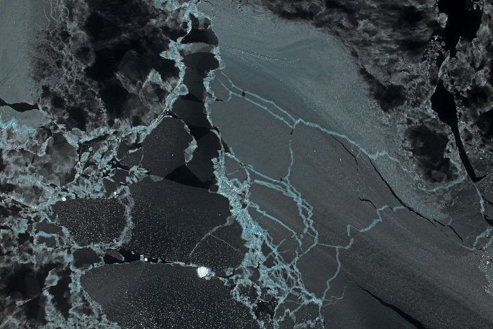
5: Thin ice between the Larsen C Ice Shelf and iceberg A-68A. (Photo by NASA/Digital Mapping System.)
After a few hours flying over the Southern Ocean and the sea ice fields around Antarctica, the first sign of land can be startling. The vast expanse of water and ice is suddenly broken by gray and brown rocky mountaintops. Ice pours down the slopes and fills hidden valleys. This is the Antarctic Peninsula, and the ice here is anything but static.
Unlike sea ice, the land ice of Antarctica has the potential to raise sea level. Most of the continent’s recent ice losses have been occurring on its western side, including the Antarctic Peninsula, the strip of land that reaches like an arm toward South America. Research has shown that the southern part of the peninsula is particularly vulnerable, as the glaciers and ice shelves there have destabilized.
To know how much and how fast these changes are occurring, IceBridge scientists have been making regular measurements in the area since 2009. These photographs were acquired on November 3, 2017, during an flight over the southern Antarctic Peninsula. The top photograph, shot by IceBridge project scientist Nathan Kurtz, shows the Creswick Peaks, which jut from the peninsula’s southwestern side just east of George VI Sound.
The rest of the photographs were acquired that day by the DMS. The photos show some of the places on the peninsula where ice flows around mountains, and where mountain tops and edges stand out in stark contrast from the snow and ice.
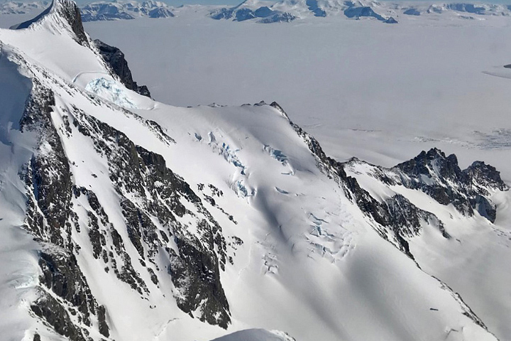
6: Snow and ice on the Creswick Peaks. (Photo by NASA/Nathan Kurtz.)
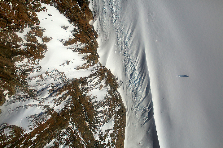
7: Ice meets mountaintops on the Antarctic Peninsula. (Photo by NASA/Digital Mapping System.)
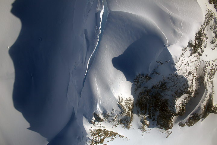
8: Mountains of the southwestern Antarctic Peninsula cast shadows on ice. (Photo by NASA/Digital Mapping System.)
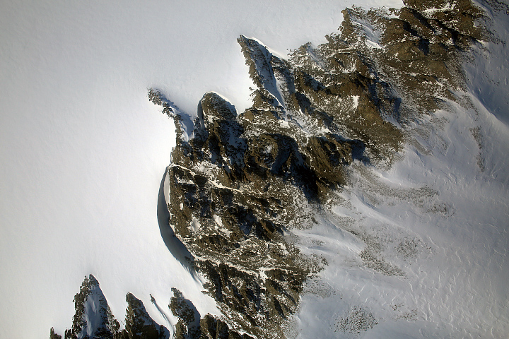
9: Stark contrast between land and ice on the Antarctic Peninsula. (Photo by NASA/Digital Mapping System.)
During any given IceBridge flight, you can see areas of fractures and crevasses that attest to lumbering motion of huge slabs of ice. Its thickness on this part of the continent can vary dramatically, from no ice at all (barren bedrock) to more than a kilometer thick. The reason for the brittle appearance is similar to the phenomenon of river rapids, which become amplified as water flows through steep, narrow terrain. As ice flows through narrower areas and steeper bedrock, more fractures open up at the ice surface. But the flow of ice is so much slower than water, and fractures are often the only perceptible indication of movement. These images, acquired by the DMS on November 3, 2017, show cracks in the ice as observed while flying over the southern Antarctic Peninsula.
The first image shows ice flowing into the southern part of the George VI ice shelf, south of the Seward Mountains in Palmer Land. The cracks are likely a semi-permanent feature of the landscape that occurs as ice flows over the bedrock. Ice flow is likely relatively slow even on this steeper part of bedrock; most of the ice loss from this part of the shelf is happening at its northern end.
The second image shows a heavily crevassed glacier, about 13 miles long and 7 miles wide, flowing west from the Dyer Plateau to George VI Sound. The north side of this glacier merges with Meiklejohn Glacier. The third image shows a heavily crevassed glacier north of Creswick Peaks that also flows west into George VI Sound.
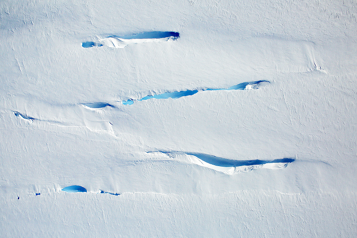
10: Semi-permanent cracks on the Antarctic Peninsula. (Photo by NASA/Digital Mapping System.)
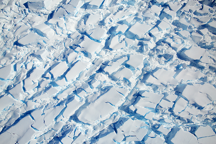
11: A heavily crevassed glacier flows west from the Dyer Plateau. (Photo by NASA/Digital Mapping System.)
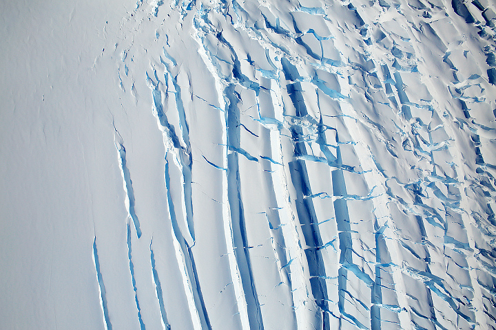
12: A heavily crevassed glacier north of the Creswick Peaks. (Photo by NASA/Digital Mapping System.)
alert message
