When astronauts talk about viewing Earth from space, the conversation often turns to the planet’s mesmerizing beauty. They describe views of aquamarine coral reefs glimmering amidst the deep blue ocean; of armies of sand dunes marching across deserts; of clouds and lightning flashes dancing through the atmosphere.
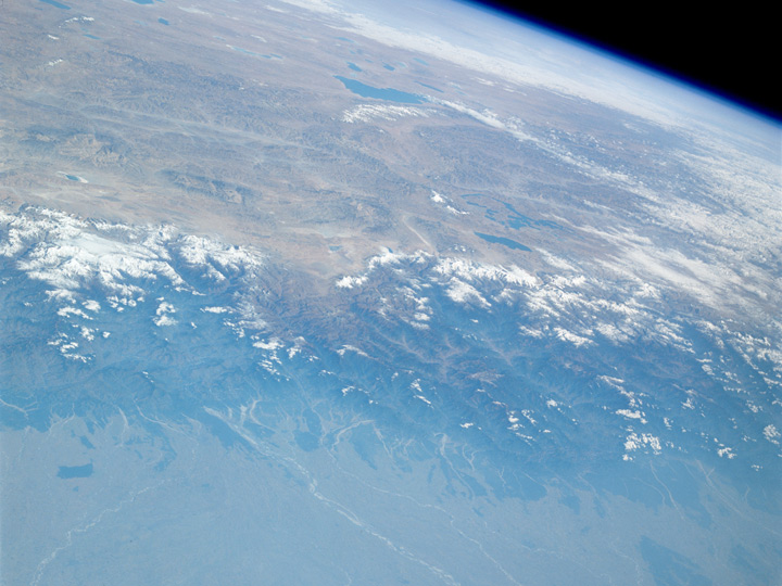
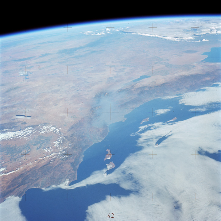
The crew of Space Shuttle Columbia captured this view of the edge of the Earth’s atmosphere, the Himalaya, and haze over Bhutan and India in late 1983. (NASA astronaut Photograph S09-41-2792).
For many, the view is deeply humbling. “For the first time in my life, I saw the horizon as a curved line. It was accentuated by a thin seam of dark blue light: the atmosphere,” said Ulf Merbold, a German astronaut who flew on Space Shuttle Columbia in 1983. “This was not the ‘ocean’ of air I had been told it was…I was terrified by its fragile appearance.”
For some astronauts, that thin blue line has appeared quite vulnerable. Many have noticed palls of haze lingering over parts of the world, the result of millions of tiny particles drifting in the atmosphere. Aerosol particles, which can be either liquid or solid, obstruct sunlight and cause distinct and vibrant features to blend into a hazy, featureless mélange of gray.
The particles that affect visibility have many sources, some of them natural. For instance, winds blow bits of dust and dried soil aloft; volcanoes occasionally belch thick plumes of ash; forest fires produce smoke; even vegetation and plankton can emit substances that contribute to haze.
But many of the particles are the result of human activity. Coal-burning power plants, smelters, and other industrial sources can produce sulfur dioxide gas, which reacts in the atmosphere to produce light-scattering sulfate particles. Combustion engines (mostly vehicles) release nitrogen oxide, which can form nitrate particles. Diesel vehicles, wood stoves, and cook stoves emit sooty black carbon. And while aerosol particles have the biggest impact on visibility, certain gases contribute to air pollution and harm human health. Ozone and sulfur dioxide, for instance, are mostly invisible to human eyes but noxious to the lungs.
From the time of the first weather satellites and human space flights in the 1960s, there were hints of air pollution. Some of the first arrived when Air Force scientists began to notice “anomalous gray shades” over the oceans as viewed by Defense Meteorological Satellite Program satellites. In 1965, Gemini VII astronauts took one of the first photographs of industrial air pollution from space. It wasn’t much to look at—a few faint smudges emanating from an otherwise grainy image of Galveston Bay, Texas.
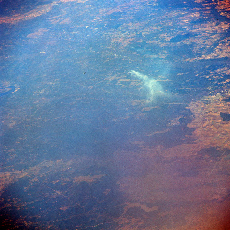
This photograph of smoke from a Louisiana sawmill is one of the earliest observation of air pollution from space. It was taken on December 6, 1965, with a description that reads “very hazy.” (NASA astronaut photograph GEM07-22-63802.)
Five decades later, the signs of air pollution are much clearer. Dozens of satellites now orbit Earth, and some of them collect information about polluting particles and gases. “In comparison to those first glimpses, the imagery and data we're getting back now are akin to looking at a modern high-definition, movie-sized color television rather than an old black-and-white set with bunny ears,” said Bryan Duncan, an atmospheric scientist at NASA’s Goddard Space Flight Center and deputy project scientist for Aura, an Earth-observing satellite.
Indeed, satellites are now sending back remarkable views of pollution that an astronaut with perfect vision could never see. Many modern satellites sense wavelengths beyond the visible portion of the spectrum, so they have mapped hot spots of gaseous pollutants over cities, power plants, oil and gas fields—even shipping lanes—that would otherwise be invisible.
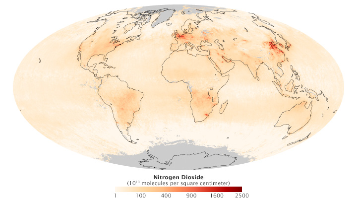
Modern satellites detect several types of air pollution. The Ozone Monitoring Instrument on Aura measured global nitrogen dioxide in September 2013. [NASA map by Robert Simmon, using data from the Koninklijk Nederlands Meteorologisch Instituut (KNMI).]
The data offer reasons for both optimism and worry. On the one hand, the once heavily polluted skies over North America and Europe have cleared considerably in recent decades due to regulations, technology improvements, and economic changes. On the other hand, satellite sensors show the opposite happening in Asia, as populations increase and countries industrialize.
Serious challenges remain. As our ability to view air pollution on a global scale has improved, so has our understanding of its widespread health consequences. According to a 2014 report from the World Health Organization, about one in eight deaths is associated with exposure to air pollution, making it “the world’s largest single environmental health risk.”
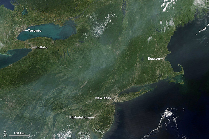
There is hope—and precedent—in today’s relatively clear skies over Europe and North America. Astronauts and satellite instruments (such as the Moderate Resolution Imaging Spectrometer (MODIS)) still occasionally see haze over the United States when pollution levels are high, but it’s rare for it to become so concentrated that the landscape below disappears. This hasn’t always been the case.
Astronaut photographs from the 1960s and 1970s contain images of thick haze blanketing the Los Angeles and San Joaquin valleys, the eastern United States, and Europe’s Po Valley. “If astronauts and satellites had had access to space prior to the 1960s, they would have seen thick smoke and haze blanketing the cities in the northeastern and midwestern U.S., particularly in the winter,” said Rudolf Husar, a Washington University atmospheric scientist who has been studying air pollution for more than forty years.
Los Angeles smog (image center), photographed by an astronaut aboard Skylab in 1973. (NASA astronaut photograph SL3-122-2591.)
During the first half of the twentieth century, coal burning at power plants, factories, and homes filled the air over the midwestern U.S. with pollution. “Smoke,” as air pollution was usually called, used to block so much sunlight that people were occasionally forced to carry lamps in the middle of the day. In some eastern cities, particulate levels likely exceeded 1,000 micrograms per cubic meter—about twice as high as they are on a bad air quality day in modern Beijing, now one of the most polluted cities in the world.
The problem was especially bad in Pittsburgh. The hills surrounding the city were filled with bitumen, a type of soft coal that released large quantities of sulfate-producing gases, soot, and other pollutants when burned. In 1866, an Atlantic Monthly writer visited Pittsburgh and reported: “The town lies low, as at the bottom of an excavation, just visible through the mingled smoke and mist, and every object in it is black. Smoke, smoke, smoke—everywhere smoke.” It was, he wrote, “like looking over into hell with the lid taken off.”
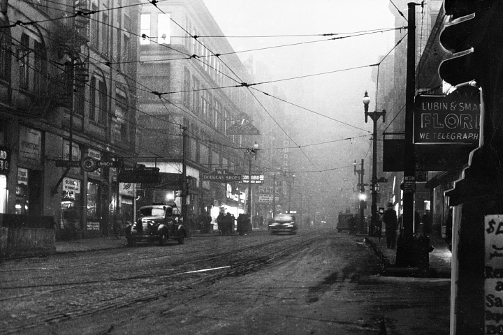
Pittsburgh’s air was often severely polluted in the mid-20th Century. A combination of the local meteorology and geography trapped smoke from the abundant steel mills in the downtown streets. (Photograph © Smoke Control Lantern Slide Collection, ca. 1940-1950, University of Pittsburgh.)
In October 1948, a disastrous outbreak of air pollution occurred in nearby Donora, Pennsylvania. What meteorologists call a temperature inversion—warmer air moving above cooler air—triggered the crisis. The warm air functioned like a lid, trapping fumes from steel and zinc smelters and exposing the town’s 13,000 residents to extremely high levels of sulfate pollution. The inversion lasted just four days, but the health consequences were swift: twenty people died and 6,000 suffered serious respiratory problems. Something similar happened in London in December 1952, leading to thousands of respiratory problems and premature deaths.
Across North America, another kind of air pollution began to plague Los Angeles, a city that burned almost no coal. Southern California was supposed to be a place of endless sunshine, but on many days a throat-burning, eye-stinging veil of smog reigned. The first severe outbreak occurred in 1943, and it baffled scientists. It had a bleach-like odor reminiscent of a chemistry lab. Plants turned yellow, wilted, and died. Strange cracking patterns appeared on tires. Headlines in The Los Angeles Times referenced a possible “gas attack” by the Japanese.
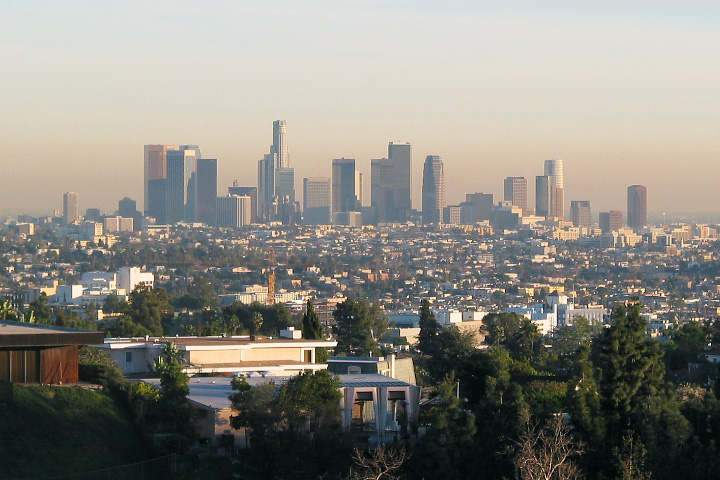
Dutch chemist Arie Haagen-Smit, known as the “father” of air quality science, finally pinpointed the source of the smog in 1950. Through laboratory experiments, he proved that the main culprit was a stew of gases coming from vehicle tailpipes. Cars and trucks were emitting volatile organic compounds and nitrogen oxides that reacted with sunlight to produce a transparent gas called ozone, the main ingredient in smog. The stew of emissions also increased levels of nitrogen dioxide, the only gaseous pollutant visible to the naked eye. The skies turned yellow-brown during extreme outbreaks of photochemical smog.
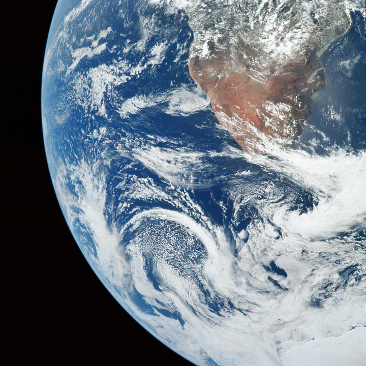
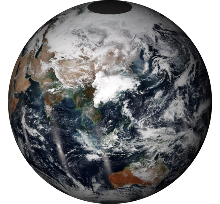
Extreme pollution outbreaks in the United States and Europe did much to put air pollution on national agendas. Satellites and astronauts accelerated the process by providing the raw imagery that helped inspire the environmental movement. As early as 1968, Stewart Brand published an image of Earth’s fully illuminated disk from Applications Technology Satellite 3 on the cover of Whole Earth Catalogue. In 1972, an Apollo 17 crewmember captured a similar shot en route to the moon. Known popularly as the Blue Marble, the photograph is perhaps the most reproduced image in human history and a global symbol of Earth’s fragility.
It all contributed to a concerted effort at local and national levels to clean up the air in the 1960s and 1970s. Coal, gasoline, and other fuels were treated or reformulated to reduce the quantity of harmful particles and gases they released. Vehicles started coming off the assembly line with catalytic converters. Regulators set limits on how often farmers could light open-air fires, and dirty cook stoves and wood stoves were replaced with cleaner-burning versions. Less-polluting fuels—such as natural gas, water, wind, and nuclear—began to take some of the load off of coal and oil-fired power plants. And those fossil-fuel power plants and factories started installing scrubbers and other emissions-filtering technologies.
While much of the work happened at the state and municipal level, efforts to clean up America’s air culminated in the 1970s with the passage of the Clean Air Act, a law that steered the United States toward better air by setting national standards for a series of key pollutants. The efforts paid off. The air over the United States today is far cleaner than three decades ago.
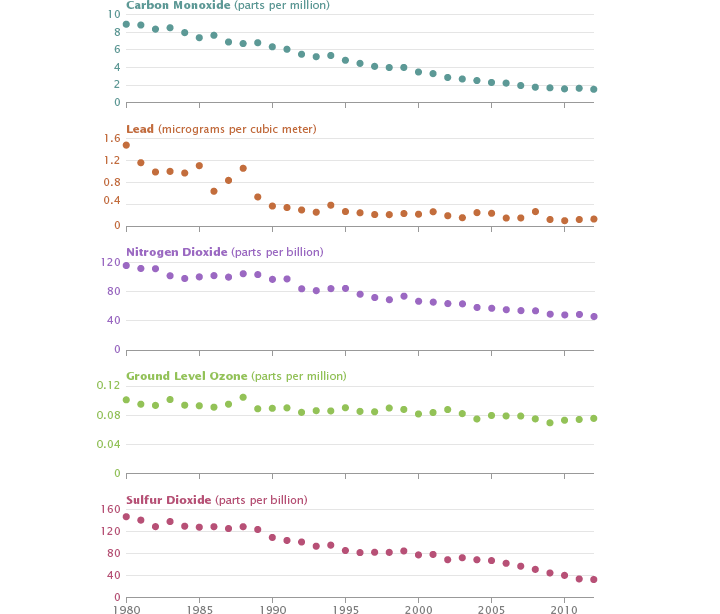
Clean air regulations in the United States have reduced the levels of 5 key pollutants since 1980. Measurements from 89 sites across the United States show the decline of carbon monoxide, lead, nitrogen dioxide, ground-level ozone, and sulfur dioxide in the atmosphere from 1980 through 2012. (Graph based on data from the Environmental Protection Agency.)
A network of ground-based air pollution sensors, operated by state and federal agencies, has measured decreases of more than 50 percent for five of the six key air pollutants regulated by the Environmental Protection Agency. Levels of lead, a heavy metal that can lead to serious neurological problems, dropped 91 percent between 1980 and 2012, mainly because of the shift to unleaded gasoline. The widespread adoption of catalytic converters led to a similarly drastic reduction in carbon monoxide (83 percent). Sulfur dioxide, which inflames lungs, has declined by 78 percent, mainly due to the installation of scrubbers on coal-fired power plants. Levels of nitrogen dioxide, a reddish-brownish gas that causes respiratory problems, fell 60 percent.
“What’s really remarkable is that the U.S. saw all of these improvements even while the population, the number of miles driven, and overall energy consumption rose,” said Duncan. “It’s an incredible achievement.”
There are thousands of ground-based monitoring stations in the United States and other industrialized nations collecting data on air pollution. But even the largest ground networks offer only a partial picture of regional and global air quality.
In North America, for instance, there are about 10 ground-monitoring stations per million people; there are just 0.4 ground stations per million people in Asia and Africa. Most ground stations are clustered around urban areas, leaving some rural towns hundreds of miles from the nearest pollution sensor. And there are huge swaths of the ocean with virtually no coverage at all.
“One of the reasons the research community has so much interest in satellites is that they will eventually be able to provide global measurements in near-real time, analogous to what weather satellites do for clouds and water vapor today,” said Jack Fishman, an atmospheric scientist at Saint Louis University who spent three decades working at NASA’s Langley Research Center.
But experts are quick to point out that satellites present their own set of challenges. It can be difficult to distinguish between pollutants high in the atmosphere and those lower down. Clouds can block measurements. And even when skies seem clear, satellites are so far away from the surface that it can be difficult to map fine details. “It’s really the integration of satellite observations, ground sensors, aerial campaigns, and computer modeling that will get us to where we need to go,” said Fishman. “But you can’t do much with the models unless you have high-quality, global-scale measurements to constrain them.”
Since the beginning of the Space Age, many sensors have been sent into orbit. However, most of them collect information about the entire column of air between the satellite and the ground. Only a small subset can measure pollutants in the troposphere, the atmospheric layer where humans live and breathe.
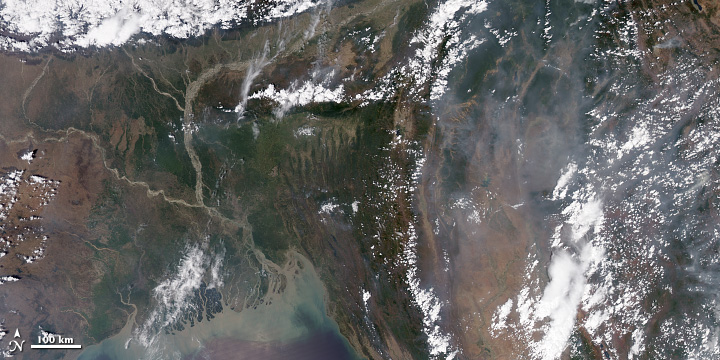
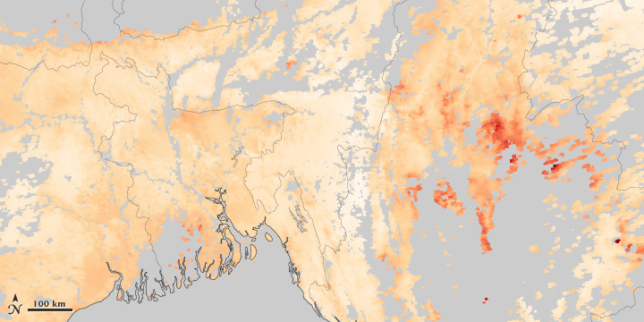
Clouds, variations between land and water, and the three-dimensional structure of the atmosphere make it difficult to measure air pollution from space. These images, collected on April 13, 2014, compare a natural-color view of of Southeast Asia to the measured concentration of aerosols. Areas of the aerosol map shown in gray indicate where the satellite could not collect valid data. (NASA images by Jesse Allen and Robert Simmon, based on data from MODIS.)
In some cases, instruments were designed to study the upper atmosphere but scientists later realized they could glean information about lower parts of the atmosphere. The Total Ozone Mapping Spectrometer (TOMS), for instance, was launched in 1978 with the goal of monitoring the ozone hole in the upper atmosphere. Scientists at NASA’s Langley Research Center later developed a technique that made it possible to retrieve information about ground-level ozone.
The European Global Ozone Monitoring Experiment (GOME-1) sensor, launched in 1995, was the first satellite instrument specifically designed to make direct measurements of gaseous pollutants in the troposphere. It measured levels of nitrogen dioxide and formaldehyde, which are good proxies for nitrogen oxides and volatile organic compounds that react in the air to form ozone. It also measured levels of sulfur dioxide at the surface.
Since then, the European Space Agency and NASA have launched more sophisticated sensors with better spatial resolution. For instance, ESA’s Scanning Imaging Absorption Spectrometer for Atmospheric Chartography (SCIAMACHY) had a resolution seven times better; the Ozone Monitoring Instrument (OMI) built by the Dutch and Finnish governments and launched by NASA on Aura, was more than 40 times better. Rather than simply measuring patches of pollution that were hundreds of square kilometers, OMI could take measurements that were on the order of a few dozen kilometers—meaning it detect elevated pollution over specific sources, such as cities or power plants.
In recent years, satellite sensors have confirmed many of the trends observed by ground-based sensors. “The real beauty of using satellites is that we can apply the same technique to the entire globe in a consistent way,” noted Nicholas Krotkov, a researcher based at NASA Goddard.
In 2011, researchers working with OMI data announced they had detected sharp declines in sulfur dioxide pollution from coal power plants in the eastern United States between 2005-2011. Although the observations only covered a short period, remote sensing scientists considered the work to be a turning point because it marked the first time such fine details about air pollution had been observed from space. The researchers—led by Environment Canada’s Vitali Fioletov, and including Krotkov—had made observations of sulfur dioxide at levels about four times lower than what had been possible before.
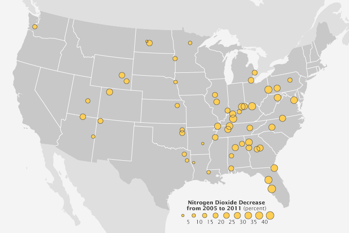
In 2013, another team used OMI data to observe a 30 percent decline in nitrogen dioxide near U.S. power plants between 2005 and 2011. The observation came just as rules went into effect requiring new emission control devices on power plants. “This type of research suggests that satellites might someday play a useful role in tracking the effectiveness of efforts to reduce pollution at individual facilities,” said Duncan.
But improving air quality in one part of the world does not necessarily mean improvement everywhere. While ground-based measurements and satellites suggest falling levels of pollution in North America and Europe, rising levels in Asia have kept the global total about the same.
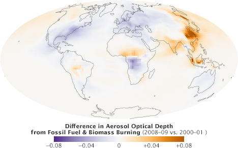
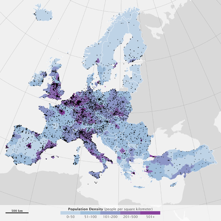
This map shows the difference in aerosol optical depth from fossil fuel and biomass burning between 2008–09 and 2000–01, as analyzed by the GOCART computer model. In general, particles released into the atmosphere by human activity decreased in the U.S. and Europe, and increased in China and India. (NASA map by Robert Simmon, using data from Chin et al. 2014.)
An analysis of satellite measurements of nitrogen dioxide levels over large cities between 1996 and 2011 is representative. Conducted by researchers from the University of Bremen, the study showed that most of the developed world—including Western Europe, the United States, Japan, and Australia—saw nitrogen dioxide levels fall as much as six percent per year. Nitrogen dioxide increased around large cities in China, India, and the Middle East, with Beijing, New Delhi, and Tehran seeing increases of 7 to 8 percent per year.
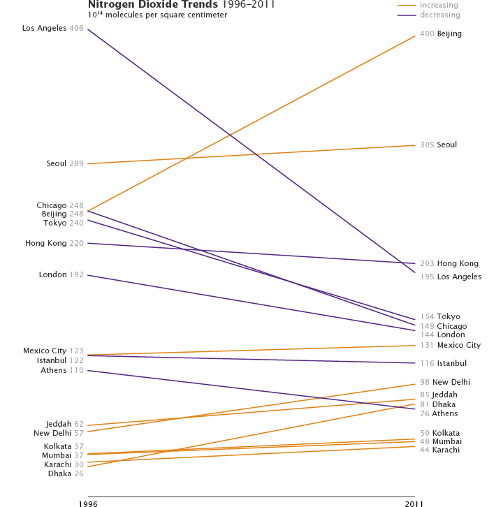
Nitrogen dioxide pollution increased strongly over cities in China, the Middle East, and India from 1996 to 2011. Western Europe, the United States, and Japan showed decreasing amounts over the same period. Monthly data shows these changes in more detail. [Graph by Robert Simmon, data provided by A. Hilboll/University of Bremen (Hilboll et al., 2013)]
Satellites that measure the distribution of aerosols have observed a similar trend. Measurements of aerosols collected by Sea-viewing Wide Field-of-view Sensor (SeaWiFS) between 1997 and 2010 showed significant increases in fine particles over India and China and decreases over North America and Europe.
In 2013, OMI helped illustrate the extent of the problem in India. Scientists using the Aura satellite observed a 63 percent increase in pollution near power plants between 2005 and 2012. However, official Indian government estimates of pollution—based on ground data collected mainly in urban areas—showed sulfur dioxide levels declining. “This implies that the air quality monitoring network needs to be optimized to reflect the true sulfur dioxide situation in India,” noted Zifeng Lu, an atmospheric scientist at Argonne National Laboratory, and his coauthors.
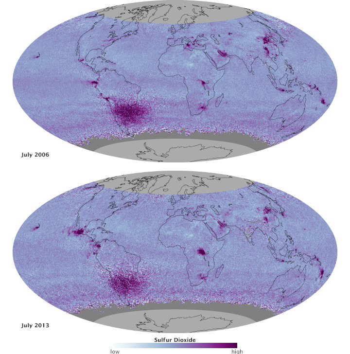
Most of the recent news out of Asia has been negative, but satellites have seen a few hopeful signs as well. After watching sulfur dioxide levels rise between 2000 and 2005, the MODIS sensors on the Terra and Aqua satellites observed a two to seven percent decrease in fine aerosols off the coast of China each year between 2005 and 2010. The authors attribute the changes to the installation of flue-gas desulfurization devices (FGDs) that reduce emissions. Only 13 percent of Chinese power plants had FGDS in 2005 but more than 70 percent had them in 2010. Likewise, an analysis of carbon monoxide data from the Measurements of Pollution in the Troposphere (MOPITT) and other sensors found a decreasing trend of about 1 percent per year in eastern China between 2000 and 2011—likely due to stricter vehicle emission standards and the phasing out of residential coal stoves.
In 2008, satellites even offered a remarkable view of how quickly the air could clear over Beijing. Due to restrictions on automobile and industrial emissions in preparation for the 2008 Olympics, levels of nitrogen dioxide over Beijing temporarily decreased by 43 percent, according to observations made by OMI.
In addition to revealing how pollution levels can change in certain areas over time, satellites have played a key role in showing how pollutants can travel from one part of the globe to another. While pollutants disperse over time and can be removed from the atmosphere by rain and other meteorological processes, satellites have occasionally observed giant rivers of pollution persisting for weeks and streaming from one continent to another. In recent years, most of these rivers had sources in Asia, flowing east across the Pacific to western North America. But satellites have also observed pollution wafting from North America to Europe, and from Europe to North Africa and Asia.
“These lines we draw on a map that separate us do not exist,” said Anousheh Ansari, an Iranian-American tourist who spent nine days on the International Space Station in 2006. “The Earth is moving all the time. There is nothing that stays constant, and there is no way you can contain a problem. The problem on the other side of the world will eventually spread.”
In 2014, a team of researchers began to quantify the connection. While it’s well known that significant amounts of dust and pollution from China end up over the United States, the researchers wanted to determine how much of that pollution from China has its origins in the demand for goods from the United States. They concluded that a significant amount—between three and ten percent—of sulfate pollution in the western United States is the result of export-related pollution from China.
“We’ve outsourced our manufacturing and much of our pollution, but some of it is blowing back across the Pacific to haunt us,” said Steven Davis, a University of California earth scientist and co-author of the study. “Given the complaints about how Chinese pollution is corrupting other countries’ air, this paper shows that there may be plenty of blame to go around.”
NASA Earth Observatory would like to thank the following people for providing content and science reviews: Ginger Butcher, Steven Davis, Bryan Duncan, Jack Fishman, Ralph Kahn, Nickolay Krotkov, Rudolf Husar, Zifeng Lu, Randall Martin, and William Morgan.
