By Eric Lindstrom
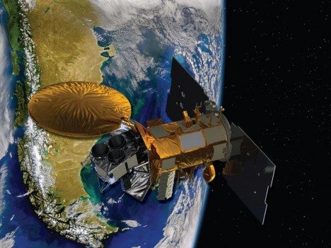
A representation of the SAC-D spacecraft, which carried the Aquarius instrument.
One of the most common questions I get (and the first comment to this blog) is “How do you measure ocean salinity from space?” During the SPURS-1 campaign in 2012 I wrote a blog post on this topic. Basically the story is one of building a very sensitive instrument (a radiometer) to detect subtle variations of L-band microwave emissions from the ocean. Aquarius, launched in June 2011 was designed specifically for that purpose. Unfortunately, the spacecraft on which the Aquarius instrument flew suffered an unrecoverable failure in spring of 2015. Fortunately for oceanography, NASA launched Soil Moisture Active-Passive mission (SMAP) in January 2015. SMAP uses similar technology (an L-band radiometer) to measure soil moisture. While SMAP is not as sensitive as Aquarius, NASA is successfully producing a salinity product from this mission’s data.
The satellite missions detect only the salinity at the surface of the ocean. This tells us much about the exchanges of water with the atmosphere once we learn how to interpret the signals. The SPURS expeditions are all about learning how the surface salinity of the ocean changes so we can use the global surface salinity maps from space to diagnose matters of the water cycle over the ocean.
The European Space Agency also launched the Soil Moisture and Ocean Salinity mission (SMOS). It uses a different technology (a synthetic aperture antenna array) to make the measurements, but also provides a salinity product we use daily. Audrey Hasson from the French space agency is aboard R/V Revelle and helping us bring all the space data (salinity, temperature, winds, sea height, waves) to the ship to guide our daily operations.
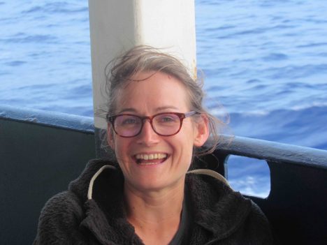
Audrey Hasson, from the French space agency, aboard the R/V Revelle.
Most of the oceanographic work on this voyage is focused on measuring and understanding the variations of salinity in the top 10 meters (~30 feet) of the ocean. Here, in one of the rainier spots on the planet, rainwater freshens the surface ocean. The degree of freshening was not really appreciated until we saw the surface salinity from space. Measurements from ships and buoys usually miss sampling the upper few meters of the ocean because it is technically difficult to make those measurements. Taking full advantage of Aquarius and SMOS surface salinity observations has required a scientific revolution in measurement of salinity in the top 10 meters of the ocean.
Getting back to shipboard life, I am happy to report that all the minor cases of seasickness are abating. Those that suffered from it are now smiling and eating. No serious cases of seasickness occurred at all, so my guess is that all the first-timers will return to sea in future!
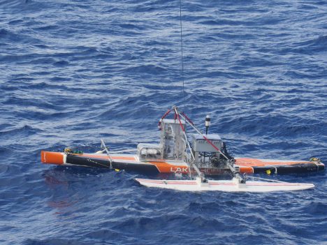
Deploying the Surface Salinity Profiler.
Also, today was the first trial deployment of one of our key instruments, the Surface Salinity Profiler (SSP), from University of Washington Applied Physics Lab. It’s a salinity measurement “laboratory on a sailboard” that can be towed at outboard of the ship. The instrument can measure salinity simultaneously and continuously at several shallow depths away from the ship’s influence and wake. The trial was devoted to the mechanics of deployment and recovery and the dynamics of towing the system. You will hear much more about SSP as the voyage progresses.
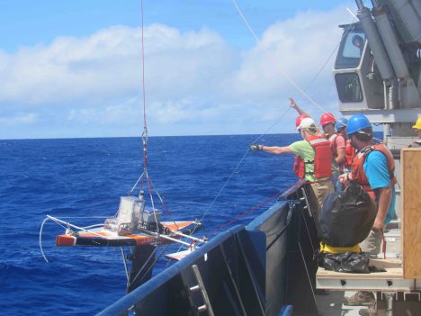
Recovering the Surface Salinity Profiler.
Winds dropped over night and whitecaps have largely disappeared. The sky is broken clouds with an occasional very light rain shower. Air temperature is 80°F. So overall, the weather conditions for test deployments off the ship are much better today!
By Eric Lindstrom
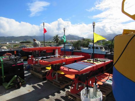
Our wave gliders, ready for action.
Fieldwork in physical oceanography, like many sciences, requires enormous preparation followed by a shorter very intensive period of action. SPURS-2 is no exception. The work over the next six weeks has been in the planning and staging for several years. Now, all the gear and scientists have reached the ship and we are on our way to completing all of our the carefully laid plans.
It is tempting to express the mood aboard the R/V Revelle as a great sense of anticipation. From discussion around the ship, it seems like no one has seen a voyage with these many sensors and equipment installed aboard this ship. There seem to be instruments mounted everywhere from bow to stern! And, of course, the scientists and technicians are deeply interested in what each sensor will tell them and what kind of scientific discoveries will emerge. These instruments are designed to see the delicate slow dance between the ocean and atmosphere around the ship over the coming weeks. Other gear will be deployed to continue the careful watch on ocean and atmosphere for the next year. All our time and investment is focused on understanding the aspects of this “slow dance” that involve water exchanges between ocean and atmosphere. In the atmosphere we will be looking at the characteristics of rainfall and evaporation at the sea surface. In the ocean we will be study the characteristics of the temperature and salinity patterns induced by the rain. These interactions are a newly accessible field of study resulting from the advent of satellite rainfall and salinity measurements and new shipboard tools for studying the upper few meters of the ocean.
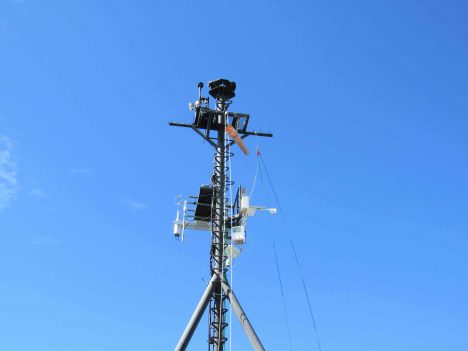
One of the numerous meteorological masts installed on the R/V Revelle for SPURS-2.
All the scientific party on R/V Revelle likely feel some sense of adventure, since the precise nature of what we will see and discover is a matter of conjecture. We do know from the Aquarius satellite data that there is a large pool of relatively fresh water built up seasonally at the surface of the eastern tropical Pacific north of the equator. Oceanographers are curious as to how this pool is trapped in the region for part of the year and how it is seasonally released to the west. As physicists, we are tackling the problem by careful examination of the individual processes that bring the water into the ocean (rain), maintain the fresh pool in the ocean (dynamics), and subsequently release the water to the west or to the deep (dynamics and mixing). If we knew the answers, it wouldn’t be research. The unknown beckons! The combined feelings of curiosity and anticipation –and that our work may result in deeper understanding of nature–, just seem to make this feel like an adventure!
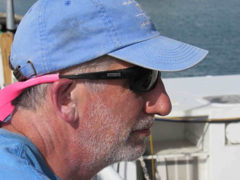
The chief scientist of SPURS-2, Andy Jessup, is ready for action too.
So here we are, all primed for discovery but with five days more to go before being where we really want to work. We are like kids in the back seat of the car asking “are we there yet?” Every piece of gear is at the ready and the teams are completing their training. We are doing dry runs to iron out the deployments of new devices that just have not seen that much action. In later entries, I’ll introduce you to the Sea Snake and the Surface Salinity Profiler and the Lighter-than-Air InfraRed System (LTAIRS), a balloon. These are very new ways of examining the air-sea interaction near the ship. They will be used in conjunction with many of our standard tools – drifters, wavegliders, and moorings, for example. We hope they will lead us to deeper insights about the water cycle at the ocean surface. I will give you a preliminary view of what is discovered during the week-long return voyage to Honolulu at the end of September. For now, we simply prepare for action!
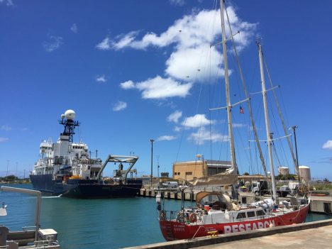
The Lady Amber and R/V Revelle in Honolulu.
By Eric Lindstrom
Two ships in Honolulu were abuzz with action this last week preparing for SPURS-2, a detailed study of ocean salinity in the eastern tropical Pacific Ocean. The Roger Revelle, upon which all the scientific party sails, had to be loaded with many tons of scientific equipment and installations completed all over the ship. Lady Amber, the 20-meter (66-feet) schooner, was also readied for action with the installation of meteorological and oceanographic gear.
It was amazing to see what was completed in only a week under the supervision of chief scientist Andy Jessup (University of Washington). Containers from Seattle, Woods Hole, and San Diego were unloaded and equipment hauled to the ships. Many scientists and technicians dedicated the entire week prior to Revelle’s departure on August 13 for stowage, assembly, installation, testing, and securing of instruments and gear. It was a very quiet ship over the last 24 hours after we departed as everyone had a well-deserved rest and acquired their sea legs!
The Lady Amber crew successfully tested its new installation of scientific gear but suffered a schedule setback when the crew discovered that the ship required a new engine prior to departure from Honolulu. These arrangements are underway and we are appreciative of the support provided by the University of Hawaii as the Lady Amber work gets completed. Lady Amber is expected to leave Honolulu in about a week and catch up with Revelle at the SPURS central work site, eight days southwest of Hawaii.
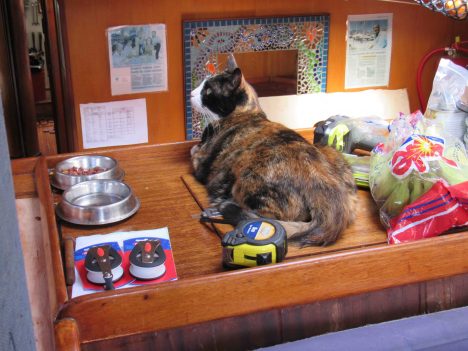
Argo the cat, relaxing in the Lady Amber.
Weather was fine on Saturday afternoon for Revelle departure. It was a quick trip out of the harbor with a great view of Waikiki skyline and Diamond Head. We passed by the Big Island of Hawaii on Sunday morning, August 14, giving people one last chance at cell phone calls. The island, really the largest mountain on our planet (from ocean bottom to summit), is a phenomenal sight.
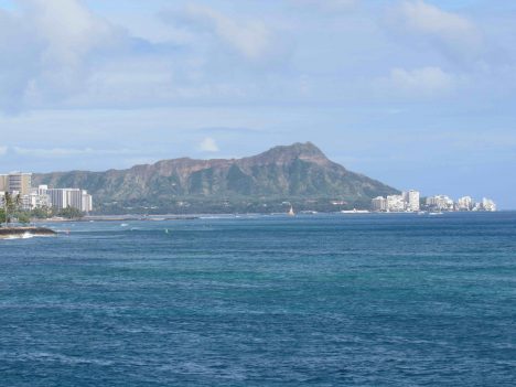
Goodbye to Honolulu!
On Sunday we had our first of weekly safety drills. Everyone got to learn how to decode the various horns that call for assembly, all clear, and abandon ship. We learned about survival suits and life raft deployment. Especially, we learned how to be safe on the Revelle and watch out for one another. We were encouraged to see the expert knowledge and conduct of the crew in their drills. It is over 2000 miles from Hawaii to the site where we begin work in earnest (deployment of moorings that pack the after deck). In the coming week, as we make the transit, the primary occupation will be testing and checking out various systems and training everyone for the complex operations to come. Once we are on site, we will quickly enter 24/7 scientific operations and we hopefully will have worked out all the glitches!
On a sad note, we had to leave our colleague Fred Bingham standing on the wharf in Honolulu, when we had expected him to sail with us. He was struck down with an illness that required he remain ashore and head home to Wilmington, North Carolina. His primary role in SPURS is as data manager. We are all assured that he will be on the mend very soon but we will miss his sunny manner and organizational skills.
The scientific party aboard Revelle is quite diverse – from first timers to old veterans. I’ll try to introduce you to the team in the weeks ahead. I am happy to report that I have seen no severe cases of seasickness during our initial day at sea. No doubt a few people are feeling a bit “green” but all are adapting well.
As always, I welcome your comments and suggestions for this blog. Send your messages to ejlindstrom@rv-revelle.ucsd.edu (case sensitive!). The expected frequency of the blog will be about one every two days.
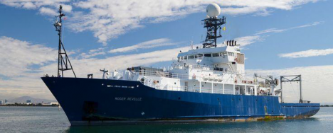
The R/V Revelle.
By Eric Lindstrom
I am writing this while on a plane headed toward Honolulu to join the Research Vessel (R/V) Roger Revelle for six weeks at sea in the Pacific Ocean. It feels great to be heading to sea again. This NASA field campaign will last more than a year, with intense shipboard work near the beginning and end of the year. A web of sensors will be deployed to monitor one oceanic region over an entire year.
As Physical Oceanography Program Scientist at NASA Headquarters for nearly 20 years, my primary job is supporting our satellite missions related to measuring physical characteristics of the ocean (principally, temperature, salinity, sea level, and winds) and supporting the oceanographers that generate knowledge from such data. True understanding requires our fully appreciating the variations of the satellite data in the context of ocean physics. And that requires getting out there and getting wet from time to time!

Your blogger, Eric Lindstrom.
R/V Revelle (home port: Scripps Institution of Oceanography, San Diego, California) leaves Honolulu on 13 August 2016 and returns to Honolulu on 23 September. The central location of the field work is about 8 days voyage southwest of Hawaii at 10N, 125W. Details of the expedition plans are available here. I hope to bring you a steady stream of expedition blog posts between now and the end of September 2016, including why NASA is focusing attention on this particular spot in the open ocean.
Since NASA’s launch in June 2011 of the Aquarius instrument to measure ocean surface salinity from space, the agency has embarked on field campaigns to understand surface salinity in great detail. This work has illuminated new ways of thinking about the ocean’s role in the global water cycle. Our field campaign, dubbed Salinity Processes in the Upper Ocean Regional Study-2 or SPURS-2, is the latest work to link the remote sensing of salinity with all the oceanic and atmospheric processes that control its variation.
The ocean is the primary source of moisture for the atmosphere. Evaporation of water from the sea surface leaves the ocean saltier (more saline). Precipitation over the ocean leaves the ocean fresher (less saline). The global pattern of average salinity at the sea surface approximately represents the balance of evaporation and precipitation at any locale (other factors such as river runoff, ice melt, and ocean motion and mixing complicate the picture). Many details of the interaction between ocean and atmosphere that lead to moisture transfer and signatures in ocean salinity are poorly understood. SPURS-2 is particularly focused on how, in one of the rainiest places on Earth, rainwater enters and impacts the ocean. Through this blog during the coming month, you will hear more about how and why oceanographers focus on such a problem.
The first SPURS campaign, which took place in the North Atlantic Ocean in 2012-2013, focused on the study of ocean processes where evaporation dominates the salinity of the surface ocean. I blogged during the September 2012 work from R/V Knorr. Among other things, we learned that surface salinity variations in that part of the world can be directly connected with precipitation patterns over the nearby continents. I’ll discuss that scientific finding and others in this blog over the coming month.
At the opposite extreme from SPURS-1, SPURS-2 focuses on an oceanic regime where precipitation dominates the salinity characteristics of the surface ocean. The two extremes call for significantly different approaches to measuring and studying the upper ocean. We will uses many of the same tools from SPURS-1 (instrumented moorings, profiling floats, surface drifters, and gliders) but deployed in new and novel ways.
The crew and scientific party on R/V Revelle will be more than 50 in all. As you read future blog entries you will get some sense of what its like for such a group to work closely together for six weeks in the confined space of an oceanographic research vessel. Seasickness? Food? Watches? Sleep? Drama? Boredom? Sea life? You’ll find out soon and get a sense of how some oceanographers go about their work, what technologies are involved, what is discovered, and how all this impacts lives, including yours, and what you might experience if you were aboard.
By Walt Meier
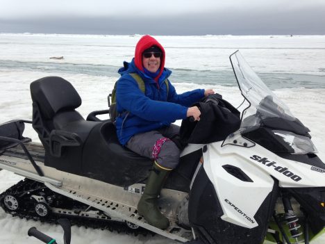
Walt Meier on a snowmobile.
May 27, afternoon – After our morning orientation and introduction sessions, I headed out onto the ice for the first time. We were split into four teams; each team will rotate through a different activity every day with each activity being led by one or two experts that will serve as our guide. I was assigned to the Red Team. Our activity for the day was sea ice morphology, or studying the forms of sea ice, and it was led by Chris Polashenski at the U.S. Army Cold Regions Research and Engineering Lab and Andy Mahoney at the University of Alaska, Fairbanks. All the other activities were being conducted within a short walk of the beach, but in order to see different types of ice, we needed to roam farther. This meant using snowmobile. After getting comfortable on the machines, we headed out. Our first stop was on a first-year ice floe, or is ice that has grown since the previous summer. This type of ice is generally thinner than multi-year ice (ice that has survived at least one summer melt season) and its thickness is largely controlled by the air temperature during the winter (though how much snow falls is important too). Colder temperatures mean more ice growth and thicker ice at the end of winter. We measured the thickness by drilling a hole through the ice using an auger. Then we dropped down a measuring tape. The tape has a folding metal bar at the end that catches the ice at the bottom of the hole; the tape is pulled taut and the thickness is read off the tape.
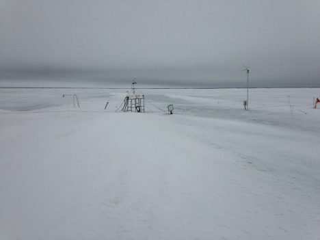
An ice mass balance station in Barrow, AK.
According to Chris and Andy, first-year ice in the area normally should be about 1.5 meters (5 feet) thick. We measured only 0.75 m. That means it’s been a very warm winter around here. But that is nothing new; in recent years, warm winters have become the norm as indicated by thickness measurements. For the past several years, Andy has been installing a sea ice mass balance station on the ice, automatically taking thickness readings every 15 minutes through the winter. The data is available online here.
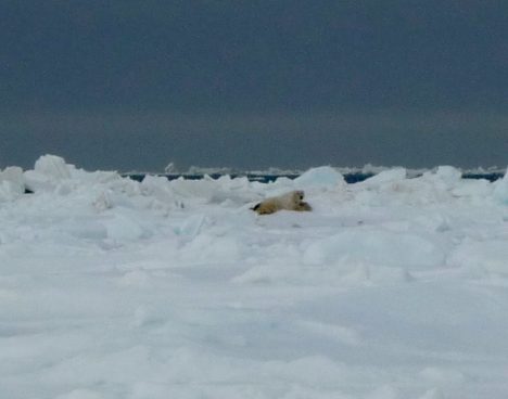
A polar bear in the distance.
Next we head further north, past Point Barrow, the northernmost land in the U.S., toward the fast ice edge. On the way, we spotted two polar bears in the distance. Polar bears are not an uncommon sight. They usually hang out near the ice edge hunting seals, though they sometimes wander into town, which can be a problem. At this time of year they are attracted by the whale carcasses that the native populations pull onto the ice as part of their traditional whale hunts. The bears were distant and barely visible, but it was quite exciting to see a bear. Polar bears can be dangerous and during all of our activities on the ice, we will have a polar bear spotter –a trained local resident carrying a shotgun – with us at all times.
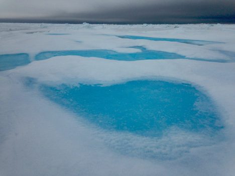
We left the polar bears to their business and rode further out to a multi-year ice floe that was more than 5 meters (16.4 feet) thick. We attempted to measure the thickness, but we didn’t break through the bottom of the ice at our auger’s (boring tool) maximum 5-meter length. To my untrained eye, the multiyear ice didn’t really look much different than first year. But with careful viewing, one could see an elevation change compared to the first-year ice. It wasn’t a lot, but a just little more elevation on the surface that floats above the ocean translates into much thicker ice because roughly 90 percent of the ice thickness lies beneath the surface of the waters. So a 5-meter thick floe of sea ice rises only about 50 cm (20 inches) above the waterline. The most distinguishing characteristic, at least at this time of year, are the brilliant blue melt ponds that form on the surface. As the snow melts, the melt water will accumulate in depressions in the ice, pooling into ponds. The crystal clear water on top of the pure multi-year ice produces a distinctive turquoise color reminiscent of the water around a tropical island. Melt ponds are very important because they absorb much more solar energy than the surrounding ice, which accelerates the melting process. But to be honest, when seeing a pond in person, the first thought one has is how pretty they are.
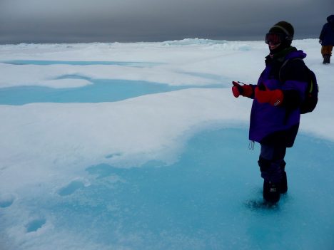
Walt, standing on a melt pond.
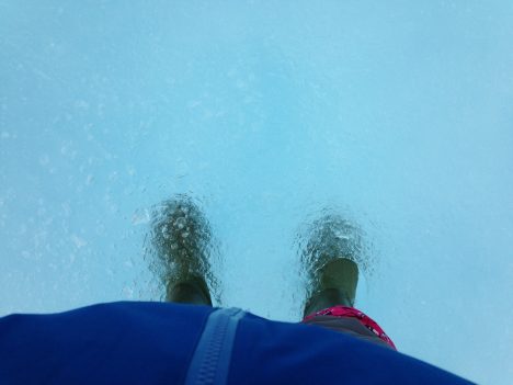
Just a few meters away, back on first-year ice, was another melt pond. But this had a much darker color due to the thinner and flatter ice. The water was also somewhat salty because first-year ice still retains some salt. The salt gets flushed out of the multiyear ice, so the blue ponds on the multiyear ice are fresh water suitable for drinking. We tried some and it was quite refreshing – ice cold!
Next, we headed over to a large piece of ridged ice. Ice ridges form due to ice floes being piled into each other due to winds or waves. The fast ice does not move, but the drifting ice beyond does and when the winds blow toward the land, the drifting ice collides with the fast ice, forming mountains of ice. The one we investigated was around 5 meters (16.4 feet) high. This means the ice could extend 50 meters (164 feet) deep below the surface. However, the water is fairly shallow off the coast and in reality, the ridge was likely grounded to the sea floor. These grounded ridges actually stabilize the fast ice by acting like big support columns, holding the fast ice in place. This explains why the coastal ice remains in place long after the drifting ice has retreated.
The morphology activity was quite humbling to us satellite data scientists and modelers. We work at scales of 5 to 50 kilometers (3 to 31 mi) – i.e., we’re observing or modeling sea ice in 5-50 km aggregates. Here over just a few kilometers we saw a tremendously varied icescape. Even over just a few meters, we saw multiyear ice, first-year ice with melt ponds on each. How can interpret our satellite data to account for such variability and how can we simulate it the models?
With the ridged ice, we completed our tour of the various forms of ice found in the Barrow area at this time of year. We hopped on our snow machines for the ride home. In front of us the sun broke through the clouds, behind us the polar bears roamed, and all around us, a lovely landscape of ice.
