Our entire team left Greenland in the last week or so and I am writing this blog post from a warm place. In this post, I will describe the additional measurements taken by the team and show a few photos to illustrate how these data were taken. As reminder, the seismic data collection was explained by Lynn here, and hydrologic measurements described by Olivia in the previous post. Here, we will present the ground-penetrating radar collection, the magnetic resonance soundings, the intelligent weather station set up, and the monitoring of the firn temperature and water-table level.
The ground-penetrating radar (GPR) was used first to decide where to extract the firn cores, do the hydrological tests, and set up magnetic soundings and seismic surveys. During the first days of the fieldwork, we did not have the snowmobile on site, so we made a small sled with a piece of foam that we could drag. It had the advantage on being light and fast to set up.
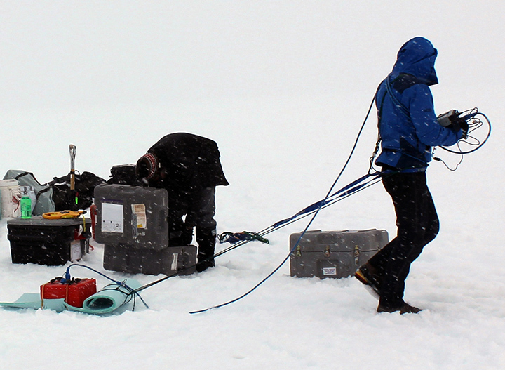
Initial GPR setup with a light sled.
The GPR profile allows us to derive the depth of the water table below the snow surface. The water table corresponds to the top of the firn aquifer and is represented in the GPR data by a bright internal horizon (see GPR profile on photo 2, bottom part). In the summer time, we expected the wet firn above the aquifer to prevent the electromagnetic signal from penetrating to the water table but we were still able to image the water table. However, the correction from two-way-travel time to depth will need to take into account the presence of near surface water as it slows down the electromagnetic signal. To determine the water-table depth and adjust our dielectrical model, the magnetic resonance soundings will be important as it provide a direct measurement of the water volume.
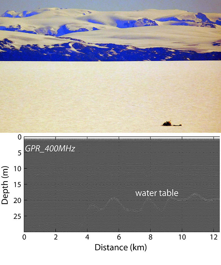
GPR survey on the snowmobile with the mountains at the background (Photo Credit: Nick Schmerr). At the bottom, example of GPR profile collected above the water table (Miège et al., 2015, JGR in review). The bright reflector represents the water table.
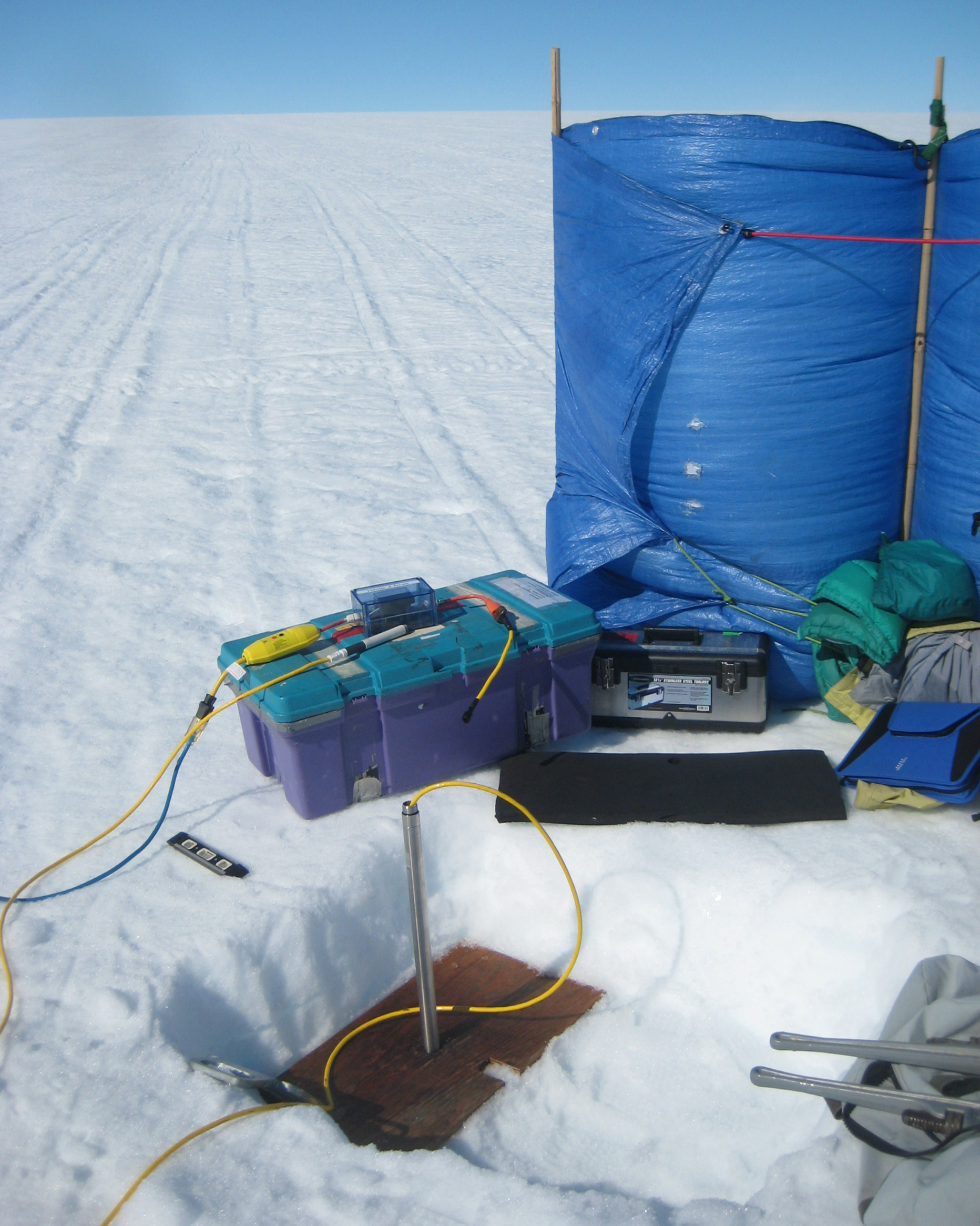
Magnetic resonance sounding (MRS) is a non-invasive technique which captures the magnetic resonance signal generated only by water molecules in the subsurface. Anatoly, a researcher from LTHE in Grenoble (FR), accepted our invitation to use his instrument over the Greenland firn aquifer. After successful initial testing in the spring, we performed several additional soundings this summer. The setup consists in a square loop about 80m long, made of wire. At one corner of the loop, all the instruments are hooked up, powered with 12V batteries.
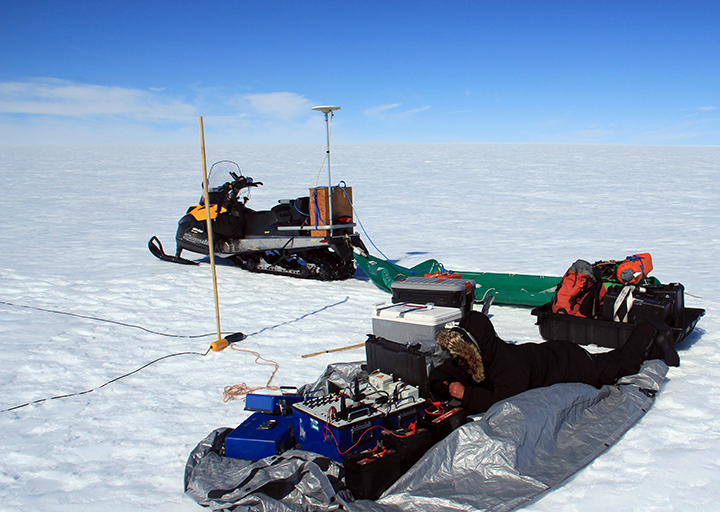
Anatoly is laying on a tarp finishing connecting the wires to the instruments. The bamboo stick marks one corner of the loop.
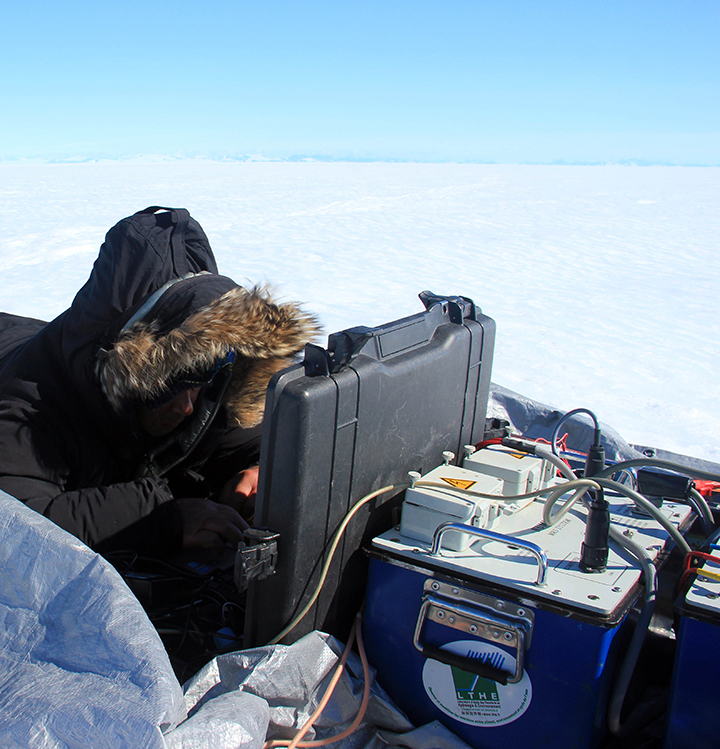
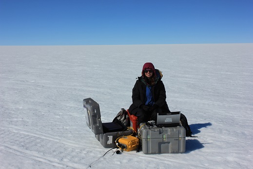
Anatoly is configuring a magnetic resonance sounding using the field computer.
One MRS takes about 1 hour to setup including walking the wire for installing the square loop. The measurement takes between 2 and 3 hours, it is always a good idea to go back to the tent for a hot drink in the meantime.
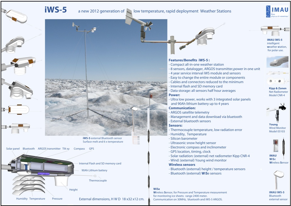
The last part of this fieldwork was to set up sensors to monitor the surface conditions on the ice sheet as well as the shallow subsurface (snow and firn) throughout the year, when we are not in the field. First, we moved the intelligent weather station (iWS) to a new location, about 20 km north. This iWS was initially installed in the spring of 2014 and we decided to move it at the new fieldwork location located directly upstream of Helheim Glacier.
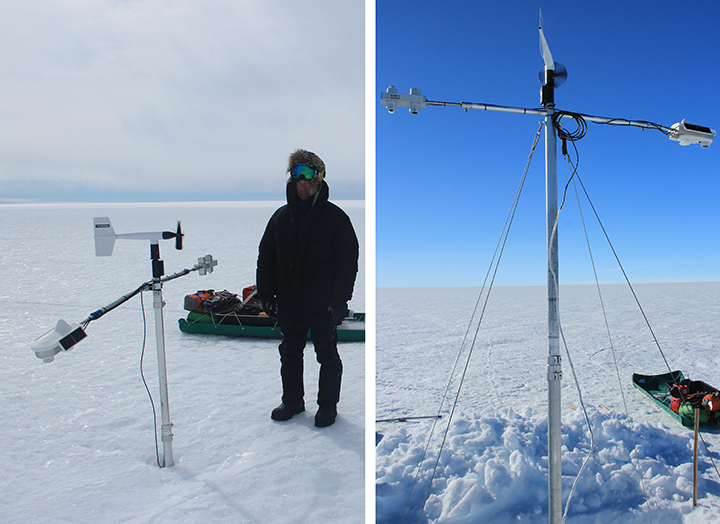
iWS developed by our colleagues from the University of Utrecht in the Netherlands. On the left, iWS at the old location and on the right, the iWS left at its new location.
To look at the firn and water thermal properties we also installed a string of 50 temperature sensors from the surface to the top of the aquifer, within the aquifer, and beyond in the ice. We also dropped a pressure sensor to measure the vertical fluctuations of the water table from the snow surface. Finally, we had the chance to use one of the compaction devices designed by our colleagues from the University of Colorado. The Colorado team is setting up the largest snow/firn compaction network on the Greenland ice sheet. If you are interested to know more about their work, follow this link. The compaction device consists of a wire with one end anchored at depth in the firn. The other end of the wire, located at the surface, reels back on a spool as the surface is lowering with snow being compacted.
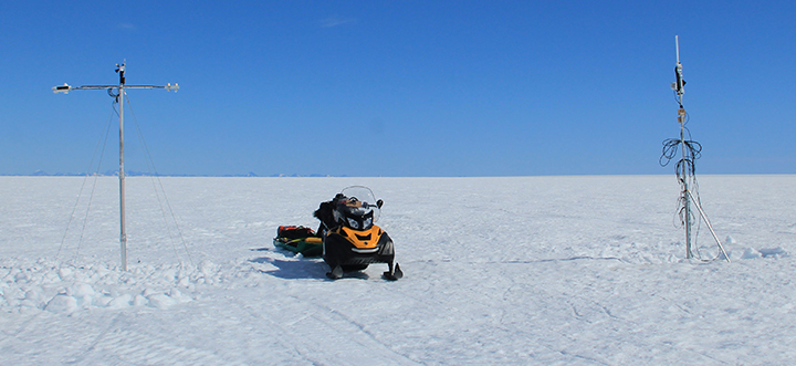
iWS standing next to the firn and water level logging station with our snowmobile in between for scale.
One of the logging stations was set up in April this year, and surprise, we got some visitors! They left us a note in the logging station case. It was a fun and unexpected moment as visitors are very rare on the ice sheet. Also it would be difficult to spot such a tiny station unless you go right by it, due to the surface undulations. These visitors are researchers from the University of Berlin, Germany. They are crossing the ice sheet between Tasiilaq and Ilulissat, repeating a route that a Swiss explorer, Alfred de Quervain, took in 1912.
Hi to them, and best of luck in their crossing! If you are interested to know more of their adventure, they left us their website link.
That is all for this blog post, stay tuned because we’ll send one last post for this summer season to wrap up and show more photos.
One of the great things about this collaborative research project is that each researcher uses very different techniques to study the firn aquifer and we will put all our results together to get the most comprehensive understanding of the aquifer. We use science techniques that look at different aspects and scales of the aquifer, from ice cores and water wells focused on single points on the ice sheet to radar, MRS, and seismic techniques that look at meters to hundreds of meters of spatial coverage. Each technique yields different, yet complementary data, particularly since we were able to use each technique at the same locations.
Installing one of two temporary wells for hydrology work.
We were incredibly lucky with the field conditions for this season and, as a result, the hydrology work went very well. The weather was the complete opposite of what we experienced in the spring. We had warm sunny days with almost 24 hours of daylight. In the spring we had issues with water freezing in the tubing we used to take water samples of the aquifer. It was warm enough that we had no problem with that this time.
Because of the good weather, we were also able to drill into the aquifer at two sites for the hydrology work. We took samples and measurements that will show us how the aquifer changes spatially. We took water samples, measured the water level of the aquifer, and did several tests to measure how quickly water moves through the firn.
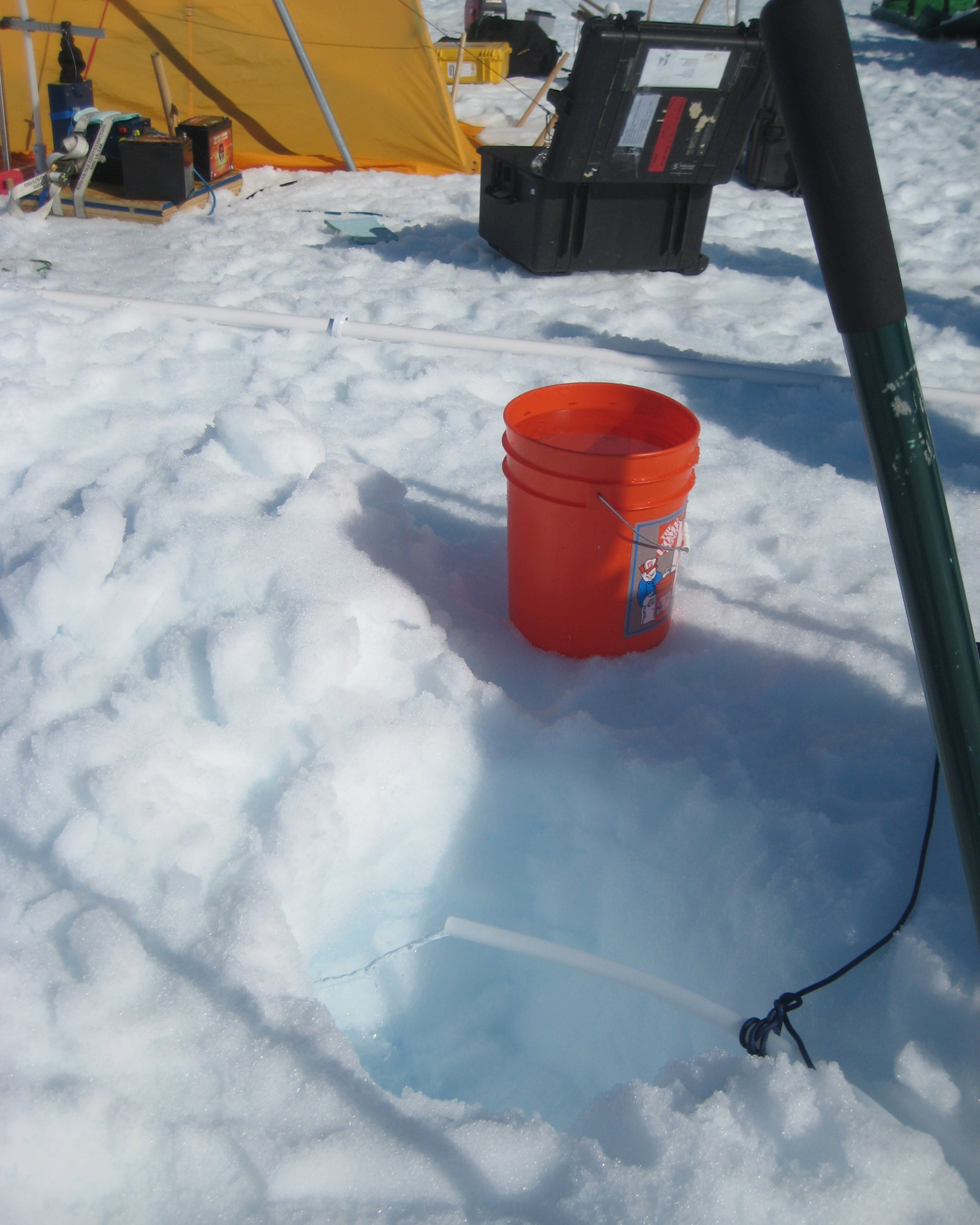
Pumping water out of the firn aquifer.
We also took samples of ice cores and water at different depths that we will measure tritium (an isotope of hydrogen that was released into the atmosphere as a product of nuclear weapons testing) in to determine how old the firn and water at each depth is. Tritium in the atmosphere was most concentrated in the 1960s and has been decreasing since them. We can measure the amount of tritium in a water sample to see how old it is. Annual layers of snow and ice preserve the atmospheric history of tritium in the atmosphere. As you drill ice cores from greater depths, you move back in time. In the spring we were really close to sampling the tritium peak so we are hoping that we drilled our ice cores deep enough to sample the peak this time.
My next steps include laboratory analysis of the samples I collected. I am looking forward to getting and sharing results soon!
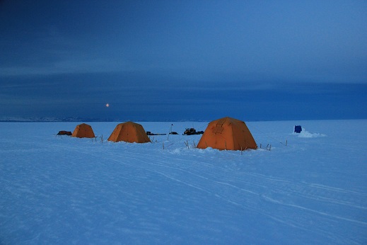
Our camp setup on a cloudy night.
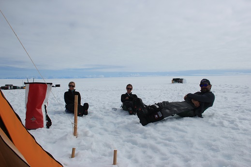
Nick, Olivia, and Lynn enjoying a beautiful afternoon with lunch outside.
After 18 long days of successful science and arctic adventures on the ice sheet, we were finally done and ready to head back to civilization. On the morning of August 13th, our expected pull out date, we received bad news from the pilots – they were not even in Kulusuk due to weather delays the day before. They planned to travel that morning and the next day to arrive so pickup should be in the coming days, however to call back later for an update. We went on with our day making pancakes and playing UNO because all the work and all the packing was complete, what else are scientists to do when all the science is done? We called the pilots in the afternoon for an update and got the best news possible – one pilot had arrived and was on his way to pick us all up that afternoon!
We headed back to Kulusuk just in time for dinner and had three sling loads come in the following days (August 14 and 15). Huge thank-you to our fantastic pilots Diddi and Johannes for the smoothest and quickest field put in/pick up so far.
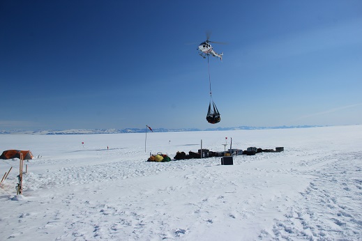
The helicopter taking in a sling load full of our gear.
This field season could not have been more rewarding and efficient. We completed all our our science goals and even got some extra data. In the field, we were able to visit all four sites as well as check out some other interesting spots near camp and near the crevasses (though still at a very safe distance!). These extra sites were chosen based on ground based radar data processed and provided by Clem in the field. The field team even got overlapping measurements of radar, seismics, MRS, hydrology, and ice core data from the same site sometimes simultaneously!

When science overlaps — Taking a seismic shot while drilling for ice cores and taking hydrological measurements of the aquifer!
The weather was perfect almost every day, we only had two days of clouds and a bit of snow overnight. The winds would moderate in the morning and generally die down in the afternoon, but wonderful conditions for working as it was not too cold. This heat would cause a bit of melt at the surface in the afternoon with no winds which would make it a bit slushy, but work was always manageable. We took no rest days, as the weather did not permit us with any spending all of our time working, some days lasting 11-12 hours. However, we do not complain about the long hours, we take this time to work in great conditions as a huge gift not often seen in Southeast Greenland especially after our last field season.
As for the seismic portion of the mission, we are very happy to report that we were absolutely successful on all fronts. Due to some logistical issues, we decided to use a smaller version of the streamer cables, the one we brought in weighs only 65 pounds instead of the 350 pound original one which also required a snowmobile to tow. We ended up doing about seventeen lines in total at 6 different sites combined. One line corresponds to a 115 meter cable with 5 meter spacing on the geophones. We took shots from 80 meters before the line and 80 meters after the line as well as on the line at ten meter spacing allowing us a much finer spatial resolution for the incoming P-waves to determine the first arrivals. That translates to over 1500 manual hammer shots and almost 600 data files. We had some very sore backs some days but the team really pitched in to help out, even slightly bending the steel hammer plate by the end! We cannot wait to analyze the data and begin looking at results.
The seismic software setup.
Here’s a video from the field showing how we collected the seismic measurements:

MODIS Rapid Response Arctic Mosaic showing the clear weather over Southeast Greenland that is enabling great field science.
The field team continues to have good weather and is ahead of schedule. They have completed the seismic and magnetic resonance soundings. They drilled into the aquifer about 15 meters below the surface and are starting hydrology measurements. All science equipment is running well and the team is in good spirits. There has only been one glitch this season so far; there was water in the fuel that was sent into the field. This has caused the generator and snowmobile to have some issues. A mechanic has been helping the team over the phone to fix the issues and over the next few days the team will be testing the reliability of the snowmobile. Currently they keep the snowmobile within 5 kilometers of camp for safety, just in case they need to walk back. No major break downs yet though, so fingers crossed. They do need to reach a site that is 20 kilometers away from camp to service a weather station. If the snowmobile is deemed unreliable they will likely use the helicopter to complete the few science goals that remain. The team may even be out of the field soon so stay tuned for lots of great field pics and commentary to come.
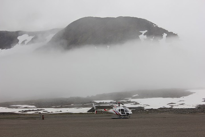
Fog rolled in over the airport with the helicopter we’ll be using in the background.
Anatoly, Nick, and I arrived in Kulusuk on July 24 after a very long journey from Maryland and France. We spent the day organizing and weighing gear from the container and are in serious need of a warm meal and good night’s sleep. This field season the seismic measurements are the top priority since they were delayed from the spring season.
The seismic portion of experiments will aid us in understanding the subsurface hydrological structure and composition of the ice sheet. These experiments are crucial for understanding how deeply the aquifer layer extends into the firn and capturing the variation in its thickness across the ice sheet. The main focus of our experiment is to use seismometers to measure the velocities of layers within the ice sheet. Based upon the various phases of water (ice, snow, and liquid water) present, we expect to see different wave speeds for each material. By examining how these wave speeds change with depth, we can deduce the relative amounts of how much water, ice, or snow is at depth.
To obtain these measurements, we will be using an active source seismic array that is being provided to us by the Incorporated Research Institutions for Seismology Portable Array Seismic Studies of the Continental Lithosphere Instrument Center. The array consists of multiple geophones attached to a towable streamer cable that will capture seismic waves propagating both along the surface and down through the ice sheet. We can move the array by towing it behind a snowmobile. To generate the seismic waves, we strike an aluminum plate with a sledgehammer to propagate a wave into the ice sheet. A single hammer strikes is typically called a “shot.” A multichannel seismic data collector connected to the seismometers then collects the ground motion recorded at each geophone, and sends the data to a computer where we can look at how long it took for the seismometers to receive data at different distances from the shot origin.
As the seismic waves travel through the ice, the time it takes for the seismometer to receive the vibration from the shot will be shorter or longer depending on the different velocities of material the wave travelled through. By looking at a number of different locations, we can then map out geographical variations in the thickness and character of the subsurface ice sheet structure. This effort is vital for understanding how water is flowing through the layers of our ice sheets in order to see how the melt is affecting sea level rise globally.
We plan on leaving for the ice sheet very soon and hope we got all of our bad luck with delays out of the way last season.
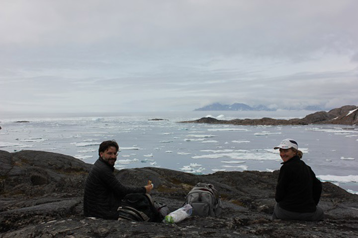
Nick and Olivia having lunch in Kulusuk.
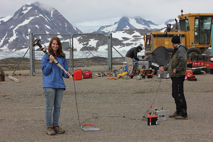
Lynn, Nick, and Anatoly testing out the seismic gear at the airport.
