My name is Mary Morris and I’m a Ph.D. candidate in the Climate and Space Sciences and Engineering department at the University of Michigan. My advisor, Prof. Chris Ruf, just so happens to be the principle investigator (PI) of the University of Michigan-led NASA Earth Venture class satellite mission, CYGNSS. CYGNSS consists of a constellation of eight satellites, scheduled to launch on December 12th. Soon! This mission will provide scientists with key hurricane ocean surface wind speed data, which we hypothesize will improve our understanding of how hurricanes form and develop. You can learn more about CYGNSS by reading earlier posts made by science team members on this blog section, or by going to nasa.gov/cygnss.
Since I have such a unique opportunity to be a CYGNSS science team member as a graduate student, I was asked to blog about my experiences in the days leading up to the launch. This has been a dream job for me and I’m excited to share my thoughts with you. In a few decades, if this blog still exists, I hope old-me will be able to look back at young-me and laugh at my wide-eyed, young scientist perspective recorded here for eternity.
So, why is working on the CYGNSS mission a dream graduate school gig? Well, I knew from a young-age that I wanted to study the weather, I just didn’t know the details of how to make a career out of my math and physics-based fascination of the atmosphere and Earth. Once I learned about remote sensing and satellite imagery, I was hooked. I knew I wanted to study more about remote sensing and eventually work on Earth science satellite missions. After a series of last minute applications to remote sensing-related research opportunities—applications that I thought were long shots—I ended up accepting Prof. Ruf’s research assistantship offer to join his remote sensing group as a Ph.D. student. The position turned out to be the graduate school jackpot: CYGNSS was selected for funding right as I started grad school. The timing could not have been better. I would get to see the inner workings of a satellite mission being developed throughout all of the design reviews and pre-launch data product development. Needless to say, it’s been an interesting ride. Since CYGNSS combines two of my passions—satellite observations and weather—it’s been a fun project to be a part of.
Graduate students are basically apprentices. If your ultimate goal is to be a scientist on Earth science satellite missions, being the graduate student working under a principal investigator of a NASA satellite mission is ideal. CYGNSS is my first satellite mission, but not my first hurricane-related research project. Here is a picture of me doing research as a part of the NASA HS3 mission (which, I also blogged about here!).
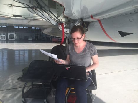
Here I am, downloading data from an aircraft instrument, HIRAD, after a science flight as a part of NASA’s HS3 mission.
I’m nearing the end of my graduate school career, and by working on both the HS3 and CYGNSS missions, I’ve gained a lot of great experience by working for and with the best engineers and scientists in our field. With the CYGNSS launch coinciding with the end of my graduate school journey, I can’t help but be a bit emotional at the end of one journey and the beginning of another.
Stay tuned for more updates throughout the weekend.
Go CYGNSS!
Numerical weather prediction models can be run with CYGNSS data included before the satellites are even in space. This is the premise behind the Observing System Simulation Experiment, or OSSE. In an OSSE, simulated measurements from any observation platform (past, present, or future) can be assimilated into a model and their impact can then be evaluated by comparing forecasts made with and without those measurements. For an introduction to CYGNSS and how it works, please read this previous blog post.
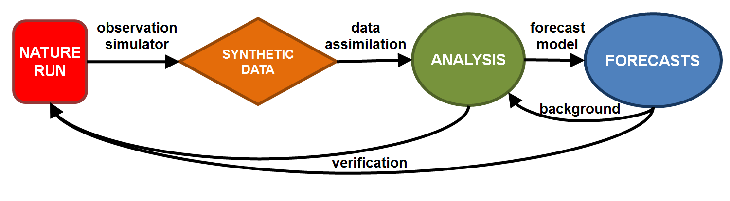
Idealized flow chart of an OSSE.
In an OSSE, the “real world” is actually high-resolution, high-quality model output from a “nature run”. That nature run is the foundation from which all observations are simulated and against which all analyses and forecasts are verified. Since the observing characteristics of instruments are known, “synthetic data” from any existing or future observation platform can be interpolated from the nature run and assigned realistic errors. If you’re living in the nature run, those synthetic data would be what your instruments would measure… including radiosondes, satellites, aircraft, buoys, and yes, even ocean surface wind speed retrievals from CYGNSS. [Note that times, dates, and events associated with the nature run are arbitrary — they do not coincide with specific events in the real world.]
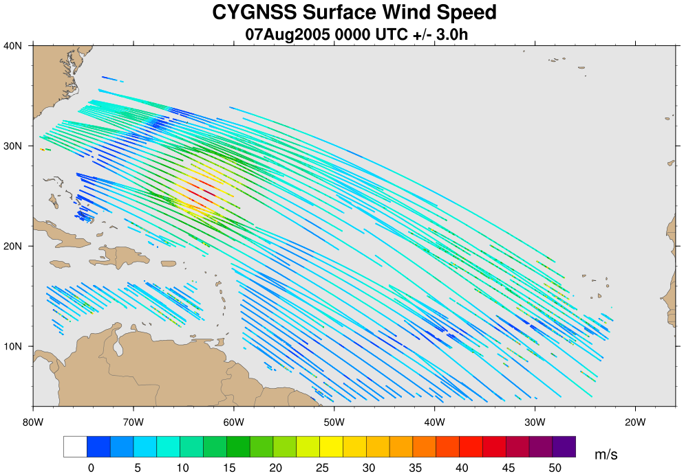
An example of synthetic CYGNSS wind speed data spanning a six hour period over the Atlantic Ocean. A hurricane can be seen north of the Lesser Antilles.
Then, the suite of observations are made available to a data assimilation (DA) system. While there are a variety of DA flavors, the basic idea is that all available observations are taken into consideration in an optimal and dynamically-consistent way to produce a best guess of the current state of the entire atmosphere. This is called the “analysis”.
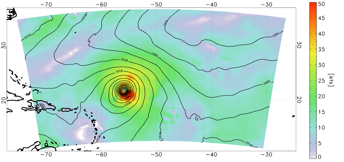
Analysis of the surface wind speed (shaded) and surface pressure (lines) on August 5 at 0000 UTC. The data assimilation method used here was a 3-D variational analysis scheme called GSI. This includes all available CYGNSS data within +/- 3 hours of the analysis time, as well as many other conventional data types.
The analysis provides the initial state for a forecast model. The forecast model, which must not be the same model used to generate the nature run, is integrated out in time. A short-term forecast (e.g. 6 hours) is used as the “background”, or first guess, for the next cycle’s analysis. Typically, the further out a forecast is run, the more it deviates from reality due to model errors, observation errors, and chaos.
The forecast model is used to produce a “control run”, which is one that includes a fixed set of observations or has a particular model configuration. Any additional data or tweaks to the DA/model system would be used to generate different runs, or experiments (“what happens if we add this”, or “what happens if we change that”). The model run is verified against the nature run by calculating errors in the analyses and forecasts — remember, the nature run is the real world in an OSSE. Output from each of the experiments can be compared to the control run to test if the errors were reduced or increased. Ideally, the addition of a new observation type such as CYGNSS improves upon the control run, but it is not always so simple in practice.
The plots below show errors in peak surface wind speed, minimum central pressure, and track for a tropical cyclone in the nature run from a control run (black line) and a single experiment with realistic CYGNSS data (red line). All of the errors from twelve forecast cycles are averaged together at the analysis time (0 hour), at 6 hours, and so on out through 120 hours. This is only an example from a single experiment, but other experiments conducted by our team include varying the DA cycling frequency, introducing “perfect” CYGNSS data interpolated directly from the nature run, adding realistic directions to the wind speeds, and assimilating higher-resolution CYGNSS data.

Errors in peak surface wind (left), minimum central pressure (middle), and track (right) for the control run (black line) and an experiment in which realistic CYGNSS data were introduced (red line). Note that lower error is ‘up’ on the y-axis on the left panel.
Based on results from a single tropical cyclone in a single nature run, simulated CYGNSS surface wind speed data do seem to have a positive impact on both analyses and short-range forecasts of tropical cyclone intensity. However, the impact on tropical cyclone track is not very noticeable, likely due to the limited influence of surface wind speeds on the storm’s steering levels.
Now we wait (im)patiently for when real data get collected and assimilated into models!
–Brian is a Senior Research Associate at the University of Miami’s Rosenstiel School of Marine and Atmospheric Science, and also blogs about hurricanes for the Washington Post.
As described in another blog post, CYGNSS is a constellation mission with eight satellites. Typically, when you launch a single satellite, you use a single rocket to put it into orbit. With eight satellites, you might think that we would use eight rockets to get them into orbit. While this would be really nice, it is not practical simply due to cost considerations.
Rockets are pretty expensive. This is primarily because there are not many of them made each year, which means that there is not a mass production facility set up to drive the prices down. There are only a few rocket launches each year, which means that each rocket is almost a custom build. The Pegasus rocket, which is one of the smallest and cheapest rockets you can get, costs about $40,000,000. Considering that the total cost of all eight satellites of CYGNSS is about $100,000,000 to design, build and test, the cost of the rocket is a lot. This means that we can’t launch each of the satellites on individual rockets, but have to launch all of them together.
In order to do that, Sierra Nevada Corporation is making a deployment module for the mission. This is a essentially a big tube that will hold all eight satellites in two rows with four satellites around the tube. When the rocket gets to just the right altitude, the deployment module will start up and deploy pairs of satellites in opposite directions. If you check out this video, you can see the deployment of the satellites. It’s a great video!
Each satellite will come off the deployment module with a speed of about 1 m/s (about 2 miles per hour) with respect to the deployment module, which will be orbiting with a speed of about 7,600 m/s (about 17,000 MPH). From one satellite’s point of view, the other satellites are moving quite slowly, while the whole constellation is moving extremely fast. For example, it will take the whole constellation about 90 minutes to orbit the Earth. For the fastest satellite to lap the slowest satellite, it will take over six months. In that time, the constellation will have gone around the Earth about 3500 times.
If you look at this video, you can see how the satellites spread out, how they lap each other, and how the global hurricane coverage changes as a function of time (as explained in this blog post). As satellites lap each other, and bunch together, the coverage dips down a little bit. While it is not a great deal, we would like to minimize this. We want to put the satellites into an evenly spaced constellation to make the coverage stay constant with time.
If the satellites were a lot bigger, they would carry propulsion, which would allow them to modify their speed. We could then space the satellites out as we would like and keep them spaced out throughout the mission. Since they are tiny microsatellites, they don’t have propulsion. But, it is possible to use the atmosphere to help up out a bit.
I recently wrote a blog post about drag and terminal velocity. In that post, I explain how air can act as a drag force on objects. Well, the atmosphere extends up into the region in which satellites orbit. In fact, the primary force that satellites feel (besides gravity) in low Earth orbit, is atmospheric drag. Satellites that are below about 500-600 km orbit, will feel such a strong drag force that they will de-orbit and burn up in the atmosphere in less than about 20 years unless they have propulsion to keep them in orbit. Above about 600 km, the lifetime of the satellites grows exponentially. (In fact, the second US satellite ever launch, in 1958, Vanguard, is still in orbit around the Earth, nearly 60 years later.)
CYGNSS will be put into orbit at about 500 km, where the drag force is quite weak (compared to here on the surface), but still exists. The satellites will de-orbit and burn up in the atmosphere in about eight years, from our calculations. Interestingly, we can change the drag force on the satellites by changing their orientation. This is because the satellites are shaped sort of like a bird – a thick center with wings. If you fly the satellites like a bird, with the wings parallel to the ground, the drag force is minimized. If you tip the satellites up, then the bottom of the wings face into the “wind” and the drag force will be increased by about a factor of eight. We can use this tipping to control the speed of the satellites and therefore the spacing. The idea is that we will tip the satellites up for a few days to change their speed a bit, then look at the constellation spacing and maybe tip a different satellite up for a while. After about six months or so of “playing” with the satellites’ orientation, drag, spacing, and speeds, they will be roughly evenly spaced around the orbital plane. Take a look at this video to see how the spacing and coverage changes when we use this concept to space the satellites out.
Using techniques like this, it is possible to launch constellations of very small satellites on a single rocket to accomplish great science!
The CYGNSS satellite mission is actually eight satellites working together as a constellation, instead of one big satellite. The good and bad of having 8 small satellites versus one big satellite were discussed in the previous post. When the mission was proposed, we had already decided how many satellites we needed to have. Deciding on eight took a lot of calculations. In this post, I would like to share with you some of the thoughts that went into these calculations.
There were a couple of important questions that we wanted to consider: (1) how much of the Earth can be measured in one day using a constellation of satellites? and (2) once CYGNSS takes a measurement over a specific point on the Earth, how long will it be before it measures that point again? These questions are somewhat related to each other, but not as much as you might expect. They are also somewhat difficult to answer, but we knew that we had to address them if we wanted the mission to move forward.
How much of the Earth can CYGNSS measure in one day?
Almost immediately, we realized that the question itself was flawed. CYGNSS would be a mission to measure winds inside of hurricanes (or tropical cyclones, to be more general). We didn’t care how often CYGNSS would measure the winds over, say, Antarctica, since there has never been a hurricane in Antarctica. We therefore started out by plotting out where hurricanes have actually occurred, which is shown in the figure below.
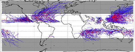
Locations of 10 years worth of tropical cyclones. The color represents the intensity of the wind speeds, with blue being weaker winds and red being stronger winds. The white section denotes where CYGNSS will orbit.
In order for a hurricane to form and grow you need two ingredients: (1) the Coriolis force, which is zero at the equator, and (2) warm water, which is most plentiful at the equator. Hurricanes tend to form and be strongest just off the equator in the northern and southern hemisphere, but not really at the equator. As they move away from the low latitudes, they lose power quickly and often die out. Therefore, there is a band around the low latitudes where the vast majority of cyclones have occurred (hence the name “tropical cyclone“).
When looking at this figure, it becomes clear that if CYGNSS goes to too high of latitude, say over Canada, then it is really just wasting time. We needed to make sure that CYGNSS stays in the tropics. And, when we calculated how often CYGNSS could measure some spot on Earth, we really only needed to care about the points where there had been a cyclone in the past, since those are the most probable locations for more cyclones.
We wrote a program that took a bunch of pretend CYGNSS satellites and a bunch of mostly-real, but virtual, GPS satellites and calculated where they would measure winds over the Earth. We broke the world up in bins that were about 15 miles by 15 miles (which is about the resolution of the winds that CYGNSS will measure), and noted which bins have had cyclones in them in the past. We then propagated the satellites around the Earth for a day and figured out all of the measurement points across the whole globe for the whole day and compared those to the bins with storms. The percentage of storm bins that had at least one wind measurement in one day is what we call our coverage. Below are some figures that show all of the measurement points across the Earth that the software computed. These are after one, two, ten and fifteen orbits (each CYGNSS satellite will orbit fifteen times in one day).
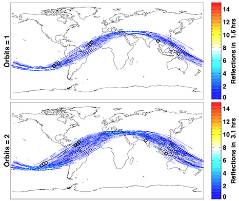
Software predictions of where CYGNSS will take measurements after one (top) and two (bottom) orbits.
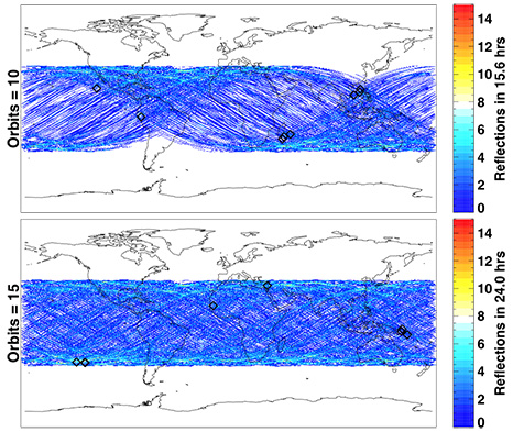
Software predictions of where CYGNSS will take measurements after ten (top) and fifteen (bottom) orbits.
Let’s take a very short break and talk about satellite orbits for a moment. If we ignore many things, we can describe a satellite orbit with a couple of numbers. The first is the altitude that it will orbit at (this is a dramatic simplification). We chose 300 miles as a hunch that it would be a good orbital altitude. And that turned out to be good for a variety of reasons, which I will explain in another post. Another very important number that controls the orbit of a satellite is the “inclination”. Simplistically, this is the maximum latitude that the satellite will pass over during an orbit. So, if the inclination of a satellite is 42 degrees, it will just reach the latitude of Ann Arbor, Michigan (42 degrees) each orbit (but won’t pass over Ann Arbor each orbit), and in the southern hemisphere, will get down to -42 degree latitude. If the inclination was 90 degrees, it would pass over the north and south poles every orbit. If it was 0 degrees, it would stay over the equator all of the time.
When I talk about not wanting CYGNSS to pass over, for example, Greenland, that means that we wanted to limit the inclination of CYGNSS’s orbit. The question was which inclination would work best? Well, with our software, we could answer this by putting in different inclinations for CYGNSS and seeing how the coverage changed. Here are some of the results:
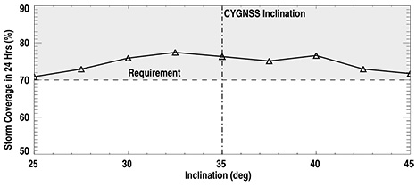
24 hour storm coverage statistics for CYGNSS given different possible inclinations for the satellites. We were wanting at least 70% coverage.
This plot shows that below about 33 degrees inclination, the coverage gets worse (i.e., lower storm coverage), and above about 40 degrees, the coverage gets worse also. We therefore chose 35 degrees, since it is a nice round number and comes over the continental United States. But, from the plot, almost any inclination between 33 and 40 would work best.
So, the answer to the first question turned out to be: in 24 hours, CYGNSS, at an inclination of 35 degrees, will be able to measure about 75% of all points on Earth where storms/cyclones have been measured before. This is very close to the capabilities of other satellites that have measured winds over the ocean. Which is good!
Repeat Times
The second question that was asked above is: Once CYGNSS takes a measurement over a specific point on the Earth, how long will it be before it measures that point again?
Since there will be eight satellites in the CYGNSS mission (which we have not even justified yet!), you can imagine having what is called a string-of-pearls: if you were to draw a string around the Earth (or put a hoola-hoop around the Earth), you could put eight satellites along that “string”. These satellites then orbit along that string, and the Earth rotates under the string. If you were to make a mark at a single point along the string, and then measure when satellites come across that line, you would get something like: 0 minutes, 12 minutes, 24 minutes, 36 minutes, etc. The satellites in the CYGNSS constellation therefore come across the point on the string every (roughly) 12 minutes.
Now, the problem is that the Earth is rotating under the string. If the mark on the string were at the equator, by the time 12 minutes has gone by, the Earth will have rotated by about 200 miles! That means that each satellite will measure a different place on the Earth when it passes through the same point in the orbit plane, simply because the Earth is rotating. If CYGNSS were orbiting over the poles, then the best we could hope for is about 12 hours repeat times, meaning that the average time between measuring the same point on the Earth would be about 12 hours. But, since CYGNSS has a 35 degree inclination, it has a very strange pattern. At certain times of the day it measures the same point a lot, while other times of the day it doesn’t measure that point at all.
This can be seen if you look at the figure above that shows 1-2 orbits. If you look at the Middle East, (virtual) CYGNSS was taking measurements in that region for both orbits. But, if you look at South Africa, CYGNSS didn’t take any measurements during those two orbits. The same was true if the south and north Pacific are compared: during the first two orbits, CYGNSS was taking measurements in the south, but not the north.
12 hours later, however, the orbit was exactly opposite, where CYGNSS took measurements over South Africa, but not over the Middle East (and the north Pacific as opposed to the south Pacific). CYGNSS tends to have a LOT of repeat measurements between about 25-35 degrees latitude (and -25 to -35 degrees latitude) during parts of the day, and no measurements during other parts of the day. Interestingly this leads to an average repeat time over the entire tropics region of about 5-6 hours, which is, on average, better than most large satellites that orbit over the poles.
These were two questions that we had to try to answer before we even started designing the satellites or even before we submitted the proposal to NASA to ask them for the money to build the CYGNSS satellites. We had to tell NASA exactly what they would be getting for their investment. All of this was leading up to the question of how many satellites do we really need to launch in order to get the measurements that help us address our science goals.
In October of 2016, NASA will launch a constellation of Micro-Satellites called CYGNSS, which stands for the Cyclone Global Navigation Satellite System. The primary science goal of the mission is to better understand how and why winds in hurricanes intensify, which is interesting from both scientific and practical points of view. CYGNSS is quite a unique satellite mission for many reasons. Over the next many posts, we will discuss how it is unique and the status of the mission.
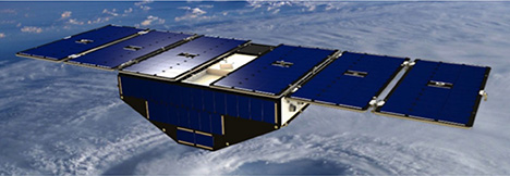
A single CYGNSS satellite. The top panels are all solar cells, except for the white strip in the middle, which contains a GPS antenna.
How Can You Measure Winds From Space?
Many missions before CYGNSS have measured winds from space using radio waves. The way this works can be explained by the analogy of looking at a full moon reflected in a lake. If you are sitting on the shore of the lake, and you see the moon reflected perfectly, then the water in the lake is extremely flat and still. This means that there is probably not much wind at all, since wind causes ripples on the lake. If the moon looks distorted, then there are probably little waves on the lake, and the wind is probably low. As the wind speed picks up, and there are more waves, the lake’s surface roughness increases, and the moon’s reflection is more distorted. If you had an instrument that only measured the total reflected brightness of the moon, you would see that decrease as the wind speed increased.
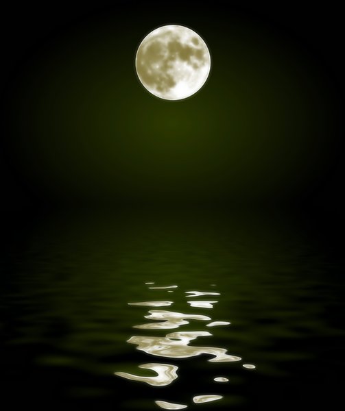
Reflection of moon off of a lake. (From http://www.rgbstock.com/bigphoto/nHepDs6/Moon+Reflected+in+Water+3)
Interestingly, if you were sitting above the lake on the opposite shore (i.e., the same side of the lake as the moon), the situation would be completely reversed: when there was no wind, the moon would reflect in a way that you couldn’t see it, but as the wind speed picked up, the moon would reflect off of the little ripples, which would allow you to see hints of it. This is called backscatter, while the other is called forward scatter. (You can read more about scatterometer techniques here.)
Most wind measurements from a satellite use the idea of backscatter to measure the amount of ripples on the oceans, which tells them the wind speed. In order to do this, the satellites have a big transmitter on board, which sends radio waves down to the surface where they are scattered by the waves. Some of those radio waves gets reflected back up (backscattered) to the satellite. Because the amount of reflected signal is quite dependent on the amount of wave activity on the ocean, the strength of the signal tells you how much wave activity is occurring. No signal means no waves, and lots of signal meaning lots of waves. Since the amount of wave activity is dependent on the wind speed, by measuring the reflected signal strength, you can deduce the wind speed.
There are a few problems with this technique, though. The first is that the satellite has to carry both a transmitter and a receiver. The transmitter is heavy, is big, and requires a lot of power, which means that the satellite has to be huge. For example, the QuickScat satellite is about 2000 pounds. Another problem is that the wavelengths of the radio waves that are used are absorbed by rain, so that the technique works well outside of hurricanes, but not within them. (The discussion of why they use these wavelengths is for another day!)
One of the brilliant things about the CYGNSS satellites is that they don’t carry a transmitter. Instead, they use GPS signals, which are being transmitted by GPS satellites all day, everyday, across the globe. Some of these radio waves are measured by your smartphone to tell you where you are, but the vast majority of the signals are just absorbed by the ground, or reflected back to space. CYGNSS measures those signals that are reflected back to space. A benefit to using the GPS signals is that those radio waves go right through rain, so that CYGNSS can take measurements in the middle of a hurricane, just where other satellites don’t work well.
Each of the eight CYGNSS satellites carry a GPS receiver onboard which measures the strength of the signal that is being forward scattered off the ocean’s surface. This is related to the roughness of the ocean and the strength of the wind. In this case, if the signal is strong, then the ocean is calm and there is not much wind, and if the signal is weak, there is a lot of wave activity, and the wind speed is strong. By not having a transmitter onboard, the satellites can be tiny – only about 60 pounds. This is allowing NASA to launch eight satellites as opposed to one. In addition, the price for those eight satellites is quite a bit smaller than the price for the single satellite. There are extremely good things about the larger satellites too, so that having both types of satellites in space allows a complementary approach to measuring the winds across the ocean and in many different types of conditions.
Over the next many posts, we will discuss other aspects of the satellites and the science behind the mission.
