By Eric Lindstrom
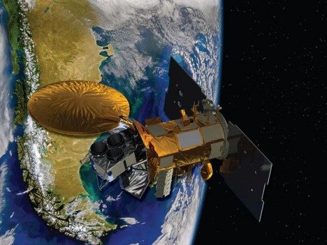
A representation of the SAC-D spacecraft, which carried the Aquarius instrument.
One of the most common questions I get (and the first comment to this blog) is “How do you measure ocean salinity from space?” During the SPURS-1 campaign in 2012 I wrote a blog post on this topic. Basically the story is one of building a very sensitive instrument (a radiometer) to detect subtle variations of L-band microwave emissions from the ocean. Aquarius, launched in June 2011 was designed specifically for that purpose. Unfortunately, the spacecraft on which the Aquarius instrument flew suffered an unrecoverable failure in spring of 2015. Fortunately for oceanography, NASA launched Soil Moisture Active-Passive mission (SMAP) in January 2015. SMAP uses similar technology (an L-band radiometer) to measure soil moisture. While SMAP is not as sensitive as Aquarius, NASA is successfully producing a salinity product from this mission’s data.
The satellite missions detect only the salinity at the surface of the ocean. This tells us much about the exchanges of water with the atmosphere once we learn how to interpret the signals. The SPURS expeditions are all about learning how the surface salinity of the ocean changes so we can use the global surface salinity maps from space to diagnose matters of the water cycle over the ocean.
The European Space Agency also launched the Soil Moisture and Ocean Salinity mission (SMOS). It uses a different technology (a synthetic aperture antenna array) to make the measurements, but also provides a salinity product we use daily. Audrey Hasson from the French space agency is aboard R/V Revelle and helping us bring all the space data (salinity, temperature, winds, sea height, waves) to the ship to guide our daily operations.
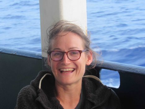
Audrey Hasson, from the French space agency, aboard the R/V Revelle.
Most of the oceanographic work on this voyage is focused on measuring and understanding the variations of salinity in the top 10 meters (~30 feet) of the ocean. Here, in one of the rainier spots on the planet, rainwater freshens the surface ocean. The degree of freshening was not really appreciated until we saw the surface salinity from space. Measurements from ships and buoys usually miss sampling the upper few meters of the ocean because it is technically difficult to make those measurements. Taking full advantage of Aquarius and SMOS surface salinity observations has required a scientific revolution in measurement of salinity in the top 10 meters of the ocean.
Getting back to shipboard life, I am happy to report that all the minor cases of seasickness are abating. Those that suffered from it are now smiling and eating. No serious cases of seasickness occurred at all, so my guess is that all the first-timers will return to sea in future!
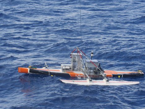
Deploying the Surface Salinity Profiler.
Also, today was the first trial deployment of one of our key instruments, the Surface Salinity Profiler (SSP), from University of Washington Applied Physics Lab. It’s a salinity measurement “laboratory on a sailboard” that can be towed at outboard of the ship. The instrument can measure salinity simultaneously and continuously at several shallow depths away from the ship’s influence and wake. The trial was devoted to the mechanics of deployment and recovery and the dynamics of towing the system. You will hear much more about SSP as the voyage progresses.
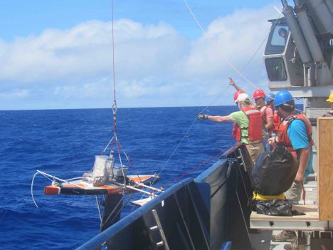
Recovering the Surface Salinity Profiler.
Winds dropped over night and whitecaps have largely disappeared. The sky is broken clouds with an occasional very light rain shower. Air temperature is 80°F. So overall, the weather conditions for test deployments off the ship are much better today!
By Eric Lindstrom
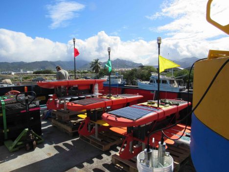
Our wave gliders, ready for action.
Fieldwork in physical oceanography, like many sciences, requires enormous preparation followed by a shorter very intensive period of action. SPURS-2 is no exception. The work over the next six weeks has been in the planning and staging for several years. Now, all the gear and scientists have reached the ship and we are on our way to completing all of our the carefully laid plans.
It is tempting to express the mood aboard the R/V Revelle as a great sense of anticipation. From discussion around the ship, it seems like no one has seen a voyage with these many sensors and equipment installed aboard this ship. There seem to be instruments mounted everywhere from bow to stern! And, of course, the scientists and technicians are deeply interested in what each sensor will tell them and what kind of scientific discoveries will emerge. These instruments are designed to see the delicate slow dance between the ocean and atmosphere around the ship over the coming weeks. Other gear will be deployed to continue the careful watch on ocean and atmosphere for the next year. All our time and investment is focused on understanding the aspects of this “slow dance” that involve water exchanges between ocean and atmosphere. In the atmosphere we will be looking at the characteristics of rainfall and evaporation at the sea surface. In the ocean we will be study the characteristics of the temperature and salinity patterns induced by the rain. These interactions are a newly accessible field of study resulting from the advent of satellite rainfall and salinity measurements and new shipboard tools for studying the upper few meters of the ocean.
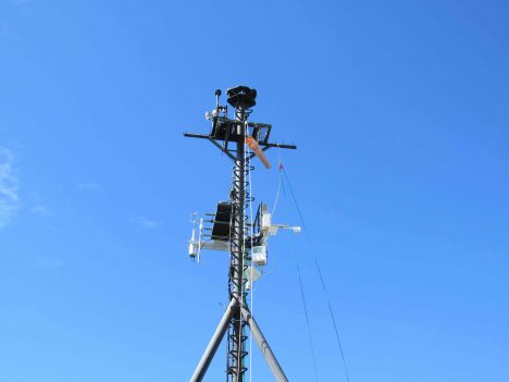
One of the numerous meteorological masts installed on the R/V Revelle for SPURS-2.
All the scientific party on R/V Revelle likely feel some sense of adventure, since the precise nature of what we will see and discover is a matter of conjecture. We do know from the Aquarius satellite data that there is a large pool of relatively fresh water built up seasonally at the surface of the eastern tropical Pacific north of the equator. Oceanographers are curious as to how this pool is trapped in the region for part of the year and how it is seasonally released to the west. As physicists, we are tackling the problem by careful examination of the individual processes that bring the water into the ocean (rain), maintain the fresh pool in the ocean (dynamics), and subsequently release the water to the west or to the deep (dynamics and mixing). If we knew the answers, it wouldn’t be research. The unknown beckons! The combined feelings of curiosity and anticipation –and that our work may result in deeper understanding of nature–, just seem to make this feel like an adventure!
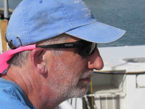
The chief scientist of SPURS-2, Andy Jessup, is ready for action too.
So here we are, all primed for discovery but with five days more to go before being where we really want to work. We are like kids in the back seat of the car asking “are we there yet?” Every piece of gear is at the ready and the teams are completing their training. We are doing dry runs to iron out the deployments of new devices that just have not seen that much action. In later entries, I’ll introduce you to the Sea Snake and the Surface Salinity Profiler and the Lighter-than-Air InfraRed System (LTAIRS), a balloon. These are very new ways of examining the air-sea interaction near the ship. They will be used in conjunction with many of our standard tools – drifters, wavegliders, and moorings, for example. We hope they will lead us to deeper insights about the water cycle at the ocean surface. I will give you a preliminary view of what is discovered during the week-long return voyage to Honolulu at the end of September. For now, we simply prepare for action!
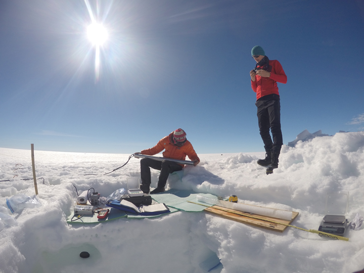
This year we teamed up with the Cold Regions Research and Engineering Lab (CRREL) (thank you Dave Finnegan and Adam Lewinter for the collaboration to produce repeat LiDAR surveys of our Rio Behar catchment primary study areas).
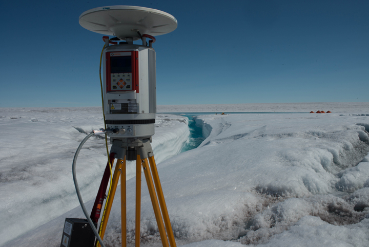
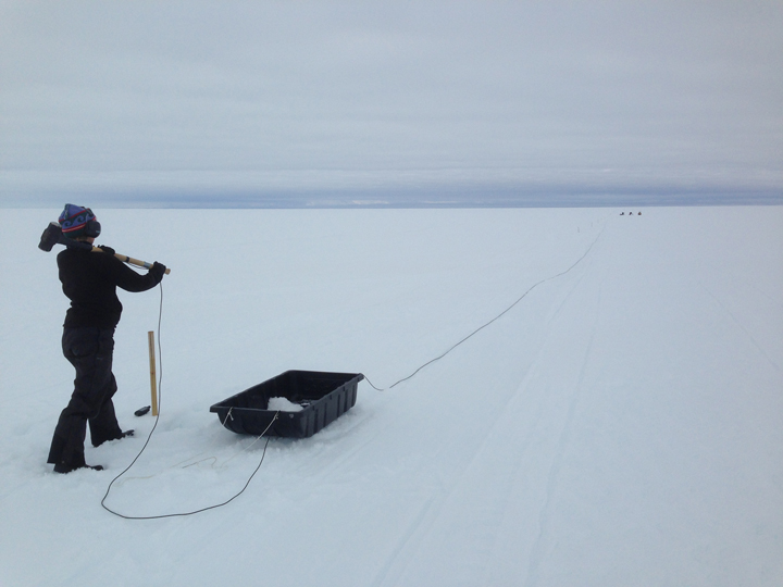
View of one of our repeat LiDAR scan locations in the Rio Behar catchment. We used a Riegl VZ-400 terrestrial laser scanner (TLS). This model is about the size of a large food processor, weighs ~40 lbs., and has a 400-600 meter range in optimal conditions. (Photo by Charlie Kershner)
LiDAR stands for Light Detection and Ranging (or, depending on where you are in the world, Laser RADAR), and it measures distances by using lasers. Basically all we’re doing is measuring the time it takes for a short duration pulse of laser light to leave the instrument, fly through the air, bounce off an object, and return to the receiver. We divide that round trip time by 2, which gives us our one-way time of flight, or the distance from the scanner to the object, and then multiply that by the speed of light, which gives us a distance. The topographic LiDAR systems we use sends out hundreds of thousands of pulses per second spaced very closely together, to build very accurate (sub centimeter) 3D models of whatever we want to image. The data we collect from these instruments is very compelling, information rich, and usually pretty easy to interpret, since it’s all in 3D and we’ve evolved to orient ourselves and understand our surroundings in three dimensions.
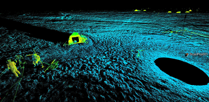
Here is a screen shot of a 3D LiDAR scan point cloud featuring one of our tents that we used to keep batteries, instruments and people warm while at ice camp.
LiDAR instruments have been used in the Arctic and Antarctic for a long time, from stationary terrestrial systems like Dave Finnegan (USACE-CRREL) and Gordon Hamilton’s (U-Maine) ATLAS project, which measures glacial flow at the Helheim Glacier, airborne systems like NASA’s Airborne Topographic Mapper (ATM), which is part of Operation IceBridge, and NASA’s Land, Vegetation and Ice Sensor (LVIS), which is now flown on its own dedicated aircraft. There are also space borne systems such as NASA’s ICESat and the forthcoming ICESat-2 mission with a planned launch date in 2017. There’s even UAV based system that we hope to fly in Greenland and Alaska soon!
There’s always a tradeoff between cost, resolution, collection rate, and collection area size. The ICESat projects can collect huge areas (nearly the whole planet), but are expensive to build and operate, and have comparatively coarser resolution. Airborne systems are cheaper than satellites and can collect higher resolution data, but flying airplanes gets expensive and are very inefficient if you want to collect small study areas at a high temporal frequency. Terrestrial LiDAR Systems (TLS) are small and comparatively inexpensive, can collect VERY high resolution data (sub centimeter) at a very high temporal resolution (same area every few minutes in order to find small-scale changes in the environment), but can be range limited and can only collect small areas (limited by the number of times you can safely pick up the scanner and physically move it from place to place).
We saw a unique opportunity to use a TLS at ice camp this year for a number of different purposes. The primary science objective was to measure the bulk ablation rate of the ice around Rio Behar. This is usually measured using ablation stakes, but measuring ablation stakes is time consuming and can be error prone. Additionally, we can’t put stakes everywhere, so we’re only able to measure ablation at specific points. We think that by using a TLS we can measure ablation at high spatial resolution over a large area, quickly, accurately, and non-destructively, providing an accurate comparison with our coincident measurements of flow in the river. The flexibility, high temporal and spatial resolution, and cost to operate made a terrestrial system a good choice for us.
We also plan to use this data to help improve the quality and assess the accuracy of other data collected during ice camp while also testing novel uses for TLS in rapidly changing cryosphere. A few additional planned uses of this data include:
We used a TLS made by Riegl called a VZ-400. It’s small, about the size of a large food processor, weighs about 40 lbs., and has a 400-600 meter range in optimal conditions. The laser operates at 1550 nanometers, in the infrared portion of the electromagnetic spectrum, which is great because it won’t damage anyone’s eyes and works well in most environments. One downside for our project is that wet snow has the same reflectance as black asphalt at 1550 nm, so our maximum effective range is more like 100 meters, not 400 meters. That’s ok though, because due to the low height of the scanner off the ground (about 6 or 7 feet), the ice hummocks in our ablation plots cause shadows in the data.
The big problem we had to solve was keeping the scanner completely motionless while collecting data. In order to measure change over time, we have to register each new scan to the scans from the day before, and we do that using a combination of aluminum cylinders with reflective tape on the outside placed in the field of view of the scanner and GPS measurements. We can use those stationary objects to tie the scans together, but only if they don’t move over the course of the week. If the tie points move, the day-to-day registration will be poor. The parameters we used resulted in each scan taking about 32 minutes to complete. If the scanner moves or shifts due to melt or wind during a scan, the data will be distorted and will have to be recollected. Stabilizing the control network as much as possible on ice in the ablation zone, which is an environment where everything is moving, required some extra work. Minimizing the amount that the tripod melted or moved in was the key to collecting the best data we could.
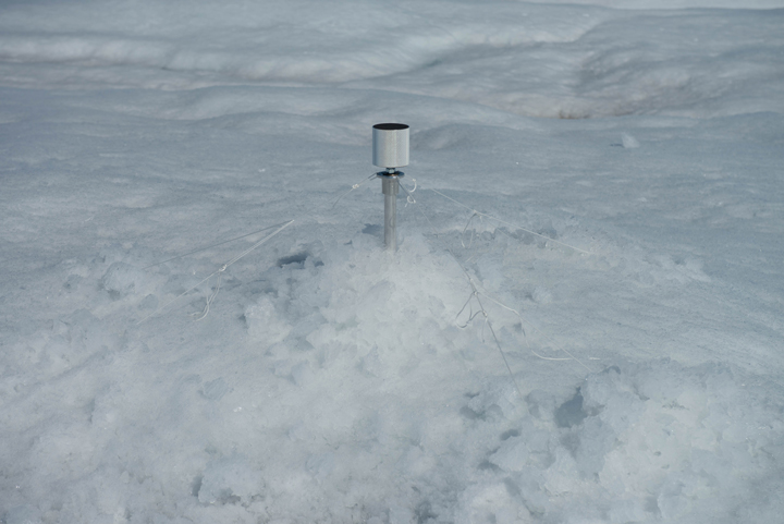
This is one of our LiDAR reflectors. We also use a differential GPS to survey the precise location of each of these LiDAR reflectors. We started all of our LiDAR scans and GPS surveys at 3 am each morning to minimize movement of the LiDAR and the GPS due to melt. (Photo by: Charlie Kershner).
The LiDAR reflectors were installed atop 2-meter-long aluminum poles drilled into the ice deep enough so only 10 or 20 centimeters remain above the surface. To add some extra stability, we tensioned the poles to the ice using cord and v-thread anchors. We stabilized the scanner and tripod by digging through the first ~20 cm of the weathering crust and securing custom engineered tripod feet to the ice with ice screws. We then buried the feet of the tripod to minimize melt around the feet (a big deal this time of year, since the sun never sets!). These feet helped distribute the weight of the scanner over a larger surface area in order to slow the rate of ablation and associated movement of the scanner.
Finally, we started collecting LIDAR data every morning at 3 am while the sun was low in the sky and temperatures were a few degrees below freezing. The cold temperatures helped in three ways: (1) the ice under the weathering crust was harder, which provided a stable surface for the tripod, (2) lower sun angles warmed the tripod legs and plywood less than they would during the middle of the day, helping minimize melt, and (3) when it was cold there was less meltwater on the ice which made the surface slightly more reflective than wet, slushy ice at 1550 nm, which gave us a little extra range with the scanner. The opportunity to take amazing photos in the beautiful light and long shadows at this time of day was an added bonus!
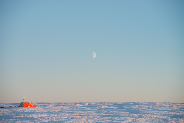
The view from the river toward our tents. (Photo by: Charlie Kershner).
Now that we’re back home, the process of data registration and processing begins. It’s not quite as much fun as collecting the data in such an amazing place, but we’re all excited to see what the data tells us about the dynamic processes in the ablation zone of the Greenland Ice Sheet.
If you want to see what LIDAR data looks like for yourself, check out plas.io or speck.ly, and interact with some sample data in a web browser. Also, GRiD and OpenTopo are two places with lots of LIDAR data from all over the world that you can download and explore.
Hi there,
After a science-packed 3 weeks on the ice sheet, the team has returned to Kulusuk, more successful than we ever expected. We accomplished the following:
First, I’ll describe a little bit about life on the ice sheet, followed by a description of the science work we did.
On a typical day, we get up around 7 and begin melting ice to make water so we can make breakfast. We generally eat instant oatmeal or, on special days, pancakes. We discuss our plans for the day and make a daily check in call to get weather updates and logistics support. This year, with 6 people in the field, we were able to divide into groups of 2 or 3. Generally, we had an ice core and hydrology team and a geophysics team. The ice core drilling and hydrology team would drill ice cores and install wells. The geophysics team did the seismic, magnetic resonance, and GPR work. Some days our work sites were in camp and we could eat a hot lunch, and other days we commuted to remote sites and packed a lunch. We had daylight until close to midnight so we often worked until 7 or 8 at night, before heading back to the cook tent to melt snow for dinner. For dinner, we eat things like pasta, couscous, or indian food that you boil in a bag. The weather was fantastic for our field work. The highs were around 5C and the lows and night were around -5C. We only had two cloudy days, which were actually a nice break from the intense sunlight we experienced the rest of the time.
Right before we went out to the ice sheet, we heard news about a polar bear entering a science camp much farther north. In response to this scary news, we beefed up our bear protection. We placed our 4 sleep tents close together, surrounded first by an electric fence and then by a trip wire that sets off a loud alarm when it is broken (I know it is loud because we had a few false alarms in the middle of the night! I have never jumped out of my 2 sleeping bags and tent so fast!) We also carried a rifle, bear spray, and noisemakers. Luckily, the only wildlife we saw was a bird on our last day on the ice.
Now for the science!This field season we had a very ambitious plan for the seismic imaging of the base of the aquifer. Based upon what we learned in last year’s field season, we wanted to investigate more of the ice lying beneath the aquifer. To do this with our seismic refraction lines, we needed to have a much longer line (540 meters vs. last year’s 275 meters). This required flipping the line of geophones after shooting the first one, and then reshooting the reversed line. Each line took 340 hammer swings to complete, with an invigorating 30 shot stack at either end being the big challenge for the hammer swingers. We also wanted a regular spacing of the seismic lines this field season; this required a bit more travel than last year on the snowmobile, with a total of 12 seismic lines spaced nearly every 2 kilometers. Some really interesting structure emerged from all this work, with in-field analysis allowing us to find the base of the water-ice transition and even see the ice-rock interface at the bed! Everyone lent an arm to the seismic work, for a total of 4120 recorded hammer swings (and a pretty dented metal plate)!
Olivia waiting for the okay to swing the hammer one more time.
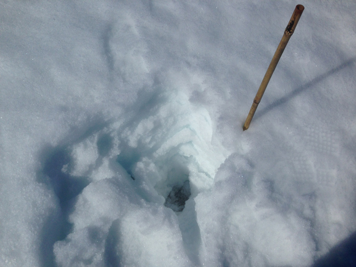
A buried plate after 30 hammer swings.
In addition to the seismic experiments, our team performed some magnetic resonance soundings and ground-penetrating radar (GPR) surveys. These two measurements combined with the seismic data help us to understand the firn aquifer structure as a whole. While the seismic measurements give us a good idea of the transition of the firn aquifer to the ice, the ice-penetrating radar was able to precisely (30 cm resolution) image the water table by sending electromagnetic waves from the surface and recording the time it takes to get them back (like a sonar on a boat). Combining seismic and radar data allowed us to get both top and bottom of the firn aquifer, therefore its thickness and its variations in space and time.
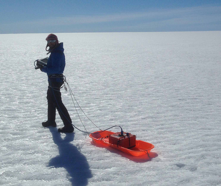
Initial GPR measurements by foot to check the presence of water and its depth. Later on we used a snowmobile to tow the radar.
The magnetic-resonance soundings (MRSs) complement the two previously described techniques by giving the total volume of free water (liquid) at each location. To measure the liquid water volume, we laid a loop of wire in a square shape, 80 x 80 m. This wire loop acts as both a transmitting and receiving antenna. For a short time, we transmit a current pulse at a known frequency through the firn and then allow the same antenna to receive the magnetic resonance response. Since only the proton in the water can generate a magnetic resonance signal at a precise frequency, we can estimate the water amount present within the wire loop.
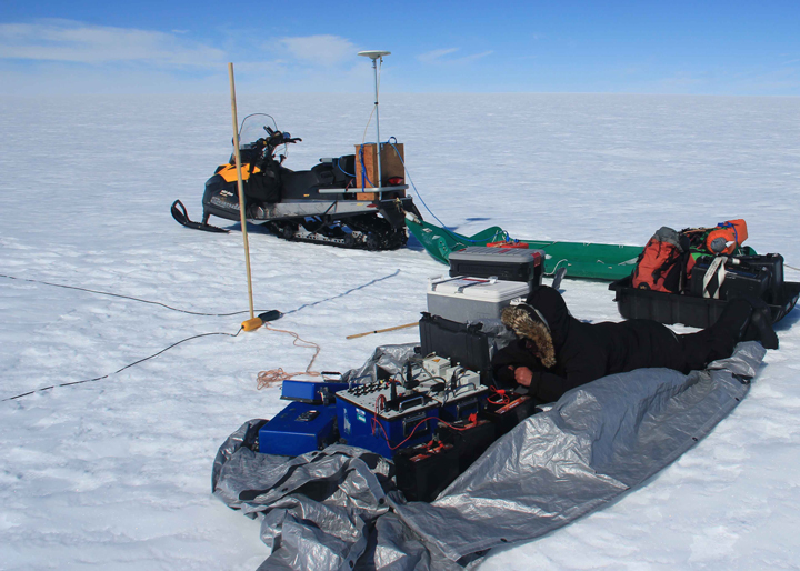
RS equipment ready for a sounding. Usually a sounding lasts between 3 and 5 hours based on how noisy the signal gets (the noisier it is, the longer the sounding takes).
Those three techniques (seismic, GPR, and MRS) complement each other nicely giving us crucial parameters to study the water present in the firn aquifer over our fieldwork location. During the 20 days in the field we were able to make 10 magnetic-resonance soundings and collect up to 100 km of GPR data, which will gives us very good spatial resolution while understanding the spread of this firn aquifer.
On the hydrology side, we installed wells and took water samples, measured permeability, and the water level like we did last year in 3 new locations. We also added a few new experiments. We did one experiments called a point dilution test where we injected salt water into the aquifer and measured how the fresh water flowing through the aquifer diluted the salt water. We can use these measurements to estimate how fast the water is flowing through the aquifer. This was really fun because we could see very quickly that the salt diluted more quickly in some parts of the aquifer than others, which tells us that the water flows at different rates in different zones.
Last summer we tried a test to measure how permeable the aquifer is called a pumping test. During a pumping test, you pump water out of the aquifer and measure how much you can lower the water table. If the water table doesn’t go down very much, it means that the water nearby can flow to the pump fairly easily. If the water table goes down a lot, it means that the water in the surrounding firn cannot flow easily enough to keep up with all the water you pump out. This summer we improved this test and were able to pump 1 liter of water per second out of the ice sheet for 5 hours! And even with all that pumping, we barely lowered the water table. This tells us that the firn is very permeable. Watch the video below to see the pumping test in in action.
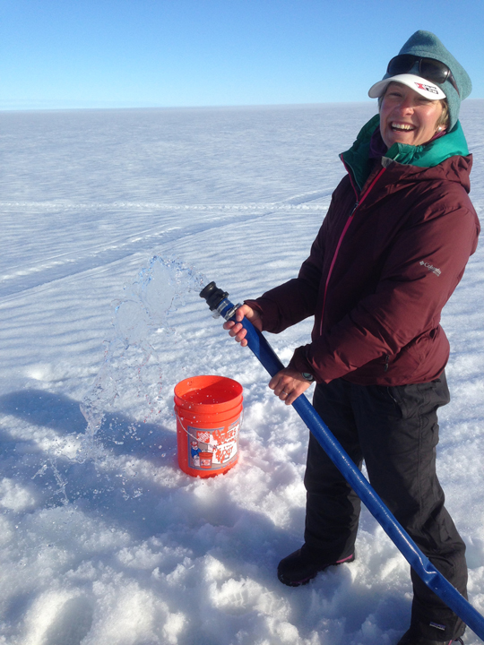
Pumping lots of water out of the ice sheet!
We also drilled ice cores at the same three sites. We measure the size and mass of each core, to determine the density of the firn and how it changes with depth. We also did a new test this year to measure the water content of the cores, and collected firn samples for chemical analysis.
Clem and Stefan studying an ice core.
All in all, we got tons of data that tells us about the aquifer structure, where the water comes from, how fast it flows, how much liquid water is stored within the ice sheet, and what impact it has on melting of the ice sheet and sea level rise.
This was a fantastic team to spend 3 weeks in isolation on the ice with! Everyone worked hard and pitched in to help each other out. We all got a chance to try doing field work for all the different kinds of science going on too. This was a really fun way to learn about other people’s work.
Now that we are back in Kulusuk, we have some work to do drying our equipment out and pacing everything up in preparation to ship it home. Time flies in the Arctic. The sun is setting much earlier, and there is a little hint of fall in the air.
On the next part of our journey the DC-8 traversed the tropical Pacific Ocean. I have always been deeply fascinated by this part of the atmosphere. The tropical Pacific Ocean lies over very warm water heated by the sun, and it is often considered to be the “firebox” of the atmosphere, the place where vast amounts of energy enter the atmosphere and drive many major features of our weather and climate.
The plane crossed two very important boundaries in the atmosphere. We encountered the first one, the Intertropical Convergence Zone (often abbreviated as the ITCZ), as our DC-8 passed 10 degrees north of the equator on the flight from Kona, Hawaii, to Pago Pago, American Samoa. The ITCZ is usually located north of the equator in Northern Hemisphere summer, and right along the equator in winter. It stands as the great meeting place between the Northern and Southern Hemispheres. Air circulates within each hemisphere in a few months, but it takes roughly a year for air to be mixed between the hemispheres by crossing the ITCZ.
I expected our measurements would see very different concentrations of pollutants as we crossed this boundary, with higher concentrations in the north than in the south. And indeed we did. The amount of carbon monoxide (CO), a major pollutant arising from all forms of combustion, dropped abruptly. But the change wasn’t as big as I expected. Other pollutants behaved the same way. The air was very clean in the northern tropical Pacific, so the North-South contrast was muted.
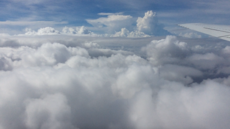
The DC-8 flies among the developing showers of the ITCZ along the equator on the flight from Kona to American Samoa. Credit: Steven Wofsy, Harvard University
But I was in for a surprise a short while later. After we had passed the ITCZ, we turned the plane to the east and travelled along the equator. Every time the DC-8 dipped down below about 10,000 feet, we saw strangely high pollutant levels, including carbon monoxide and indicators of fresh burning, such as benzene and fine particles of smoke and soot. Here we were in the midst of fresh pollution, in the Southern Hemisphere where air is supposed to be so clean. We were more than 6,000 miles from the nearest land!
Maybe I should not have been surprised. Our atmospheric computer models had actually predicted that we would see these chemicals. According to Junhua Liu, the scientist at Goddard Space Flight Center who generated the forecast, the chemicals originated in South America where fires are set each August to remove weeds and crop residues from agricultural fields and to clear trees in the forest. The goal of our ATom mission is to find out where, and how, pollutants reach the most remote parts of the planet, and we had certainly found a big input in a very surprising place, where very few people have been able to sample before us.
We encountered the second boundary, the South Pacific Convergence Zone (SPCZ) on the next flight of the DC-8 from Pago Pago to Christchurch, New Zealand. American Samoa is a lush tropical island with craggy mountains covered in jungle and clouds and generally mild weather. All that was about to change in a hurry.
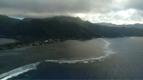
The DC-8 climbs steeply away from the tropical island of American Samoa, with its mountains covered by warm clouds. The next land we see on the ATom mission is the South Island of New Zealand, deep in winter. Credit: Bruce Daube, Harvard University.
First we came upon the SPCZ. The SPCZ is a powerful, nearly stationary feature of the South Pacific, where cold winter air from the south meets the warm, humid air from the tropics. This front is a continuous band of heavy rain and winds. Embedded in the front is the subtropical jet stream, which had winds over 200 knots (230 miles per hour) and powerful turbulence at its core the day that we were there. Our safe passage and successful sampling required close coordination between the crew and the meteorological team of ATom — Paul Newman of NASA’s Goddard Space Flight Center on the plane, and Eric Ray of NOAA’s Environmental Systems Research Laboratory on the ground.
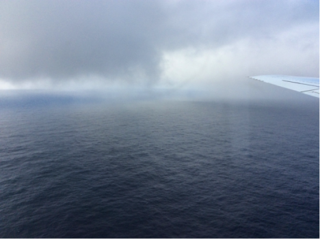
The leading edge of the SPCZ. The DC-8 sampled down to 500 feet over the ocean at the northern edge of the SPCZ, finding a view more likely to be seen from a boat than a jet aircraft. With stormy weather ahead, we took our samples quickly and climbed as high as we could. Even at the ceiling of the DC-8’s altitude, we still encountered rough flying conditions. Credit: Steven Wofsy, Harvard University
Finally, we approached the South Island of New Zealand. What a contrast to American Samoa! The mountains were clothed in snow. The valleys had been made into tidy farms with wind breaks and agricultural fields. One of the scientists on board, Róisín Cammane of Harvard, thought the farms looked just like her home country in Ireland, although the mountains are bigger.
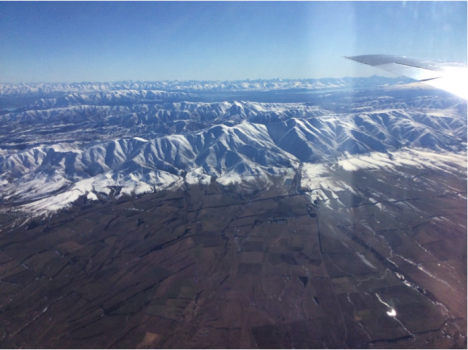
Coastal mountains on the South Island of New Zealand, near Lauder Station, overlooking agricultural lands. Credit: Steven Wofsy, Harvard University
We made a low pass over the famous observatory at Lauder, with more than 50 years of measurements of the atmosphere. A team of scientists at New Zealand’s National Institute of Water and Atmospheric Research (NIWA), led by Dave Pollard, run the station. The station is part of NASA’s Total Carbon Column Observing Network (TCCON) and hosts a spectrometer that looks at the sun and, by looking at the part of the light spectra that is known to be absorbed by carbon dioxide, measures the total amount of carbon dioxide in the atmosphere. TCCON was designed and implemented for NASA by Paul Wennberg of Caltech to help calibrate the Orbiting Carbon Observatory satellite.
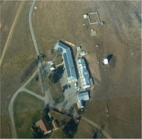
Lauder Station of New Zealand’s National Institute of Water and Atmospheric Research (NIWA). The DC-8 made a low pass over this site in order to help calibrate the TCCON measurements of carbon dioxide, which are made by looking at the sun with a spectrometer housed in the domed structure at the top of the image. Credit: Bruce C. Daube, Harvard University, from the NASA DC-8
Our aircraft measurements provide a direct link between the measurements that scientists make by sampling air at the ground and the measurements made by satellite and the TCCON looking at sunlight. On the airplane we measure samples of air, just like sampling on the ground, but we can take those samples along most of the path from the ground to the top of the troposphere, getting the total amount of carbon dioxide for the whole column, which the TCCON sites measure. My group have done these type of measurements all over the world, starting in 2004, and we have been to Lauder five times before, but never have we had such a clear day as we did on this flight.
Correction: Aug 19. The Goddard weather forecaster was misidentified in the original post. It has been corrected in the text.
