
This year we teamed up with the Cold Regions Research and Engineering Lab (CRREL) (thank you Dave Finnegan and Adam Lewinter for the collaboration to produce repeat LiDAR surveys of our Rio Behar catchment primary study areas).
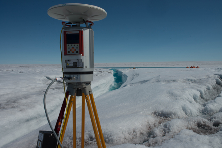
View of one of our repeat LiDAR scan locations in the Rio Behar catchment. We used a Riegl VZ-400 terrestrial laser scanner (TLS). This model is about the size of a large food processor, weighs ~40 lbs., and has a 400-600 meter range in optimal conditions. (Photo by Charlie Kershner)
LiDAR stands for Light Detection and Ranging (or, depending on where you are in the world, Laser RADAR), and it measures distances by using lasers. Basically all we’re doing is measuring the time it takes for a short duration pulse of laser light to leave the instrument, fly through the air, bounce off an object, and return to the receiver. We divide that round trip time by 2, which gives us our one-way time of flight, or the distance from the scanner to the object, and then multiply that by the speed of light, which gives us a distance. The topographic LiDAR systems we use sends out hundreds of thousands of pulses per second spaced very closely together, to build very accurate (sub centimeter) 3D models of whatever we want to image. The data we collect from these instruments is very compelling, information rich, and usually pretty easy to interpret, since it’s all in 3D and we’ve evolved to orient ourselves and understand our surroundings in three dimensions.
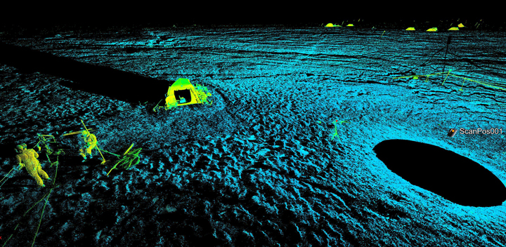
Here is a screen shot of a 3D LiDAR scan point cloud featuring one of our tents that we used to keep batteries, instruments and people warm while at ice camp.
LiDAR instruments have been used in the Arctic and Antarctic for a long time, from stationary terrestrial systems like Dave Finnegan (USACE-CRREL) and Gordon Hamilton’s (U-Maine) ATLAS project, which measures glacial flow at the Helheim Glacier, airborne systems like NASA’s Airborne Topographic Mapper (ATM), which is part of Operation IceBridge, and NASA’s Land, Vegetation and Ice Sensor (LVIS), which is now flown on its own dedicated aircraft. There are also space borne systems such as NASA’s ICESat and the forthcoming ICESat-2 mission with a planned launch date in 2017. There’s even UAV based system that we hope to fly in Greenland and Alaska soon!
There’s always a tradeoff between cost, resolution, collection rate, and collection area size. The ICESat projects can collect huge areas (nearly the whole planet), but are expensive to build and operate, and have comparatively coarser resolution. Airborne systems are cheaper than satellites and can collect higher resolution data, but flying airplanes gets expensive and are very inefficient if you want to collect small study areas at a high temporal frequency. Terrestrial LiDAR Systems (TLS) are small and comparatively inexpensive, can collect VERY high resolution data (sub centimeter) at a very high temporal resolution (same area every few minutes in order to find small-scale changes in the environment), but can be range limited and can only collect small areas (limited by the number of times you can safely pick up the scanner and physically move it from place to place).
We saw a unique opportunity to use a TLS at ice camp this year for a number of different purposes. The primary science objective was to measure the bulk ablation rate of the ice around Rio Behar. This is usually measured using ablation stakes, but measuring ablation stakes is time consuming and can be error prone. Additionally, we can’t put stakes everywhere, so we’re only able to measure ablation at specific points. We think that by using a TLS we can measure ablation at high spatial resolution over a large area, quickly, accurately, and non-destructively, providing an accurate comparison with our coincident measurements of flow in the river. The flexibility, high temporal and spatial resolution, and cost to operate made a terrestrial system a good choice for us.
We also plan to use this data to help improve the quality and assess the accuracy of other data collected during ice camp while also testing novel uses for TLS in rapidly changing cryosphere. A few additional planned uses of this data include:
- assess the accuracy of digital elevation models (DEMs) generated using photogrammetric techniques and imagery collected onboard airborne and space borne platforms
- precise geolocation every instrument, ablation stake, flag, meteorological station, and GPS base station in our study area
- take the coolest team photos ever
- and many more. . .
We used a TLS made by Riegl called a VZ-400. It’s small, about the size of a large food processor, weighs about 40 lbs., and has a 400-600 meter range in optimal conditions. The laser operates at 1550 nanometers, in the infrared portion of the electromagnetic spectrum, which is great because it won’t damage anyone’s eyes and works well in most environments. One downside for our project is that wet snow has the same reflectance as black asphalt at 1550 nm, so our maximum effective range is more like 100 meters, not 400 meters. That’s ok though, because due to the low height of the scanner off the ground (about 6 or 7 feet), the ice hummocks in our ablation plots cause shadows in the data.
The big problem we had to solve was keeping the scanner completely motionless while collecting data. In order to measure change over time, we have to register each new scan to the scans from the day before, and we do that using a combination of aluminum cylinders with reflective tape on the outside placed in the field of view of the scanner and GPS measurements. We can use those stationary objects to tie the scans together, but only if they don’t move over the course of the week. If the tie points move, the day-to-day registration will be poor. The parameters we used resulted in each scan taking about 32 minutes to complete. If the scanner moves or shifts due to melt or wind during a scan, the data will be distorted and will have to be recollected. Stabilizing the control network as much as possible on ice in the ablation zone, which is an environment where everything is moving, required some extra work. Minimizing the amount that the tripod melted or moved in was the key to collecting the best data we could.
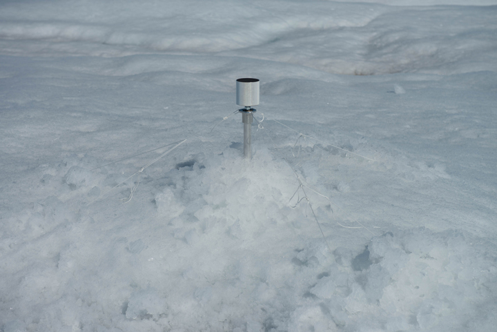
This is one of our LiDAR reflectors. We also use a differential GPS to survey the precise location of each of these LiDAR reflectors. We started all of our LiDAR scans and GPS surveys at 3 am each morning to minimize movement of the LiDAR and the GPS due to melt. (Photo by: Charlie Kershner).
The LiDAR reflectors were installed atop 2-meter-long aluminum poles drilled into the ice deep enough so only 10 or 20 centimeters remain above the surface. To add some extra stability, we tensioned the poles to the ice using cord and v-thread anchors. We stabilized the scanner and tripod by digging through the first ~20 cm of the weathering crust and securing custom engineered tripod feet to the ice with ice screws. We then buried the feet of the tripod to minimize melt around the feet (a big deal this time of year, since the sun never sets!). These feet helped distribute the weight of the scanner over a larger surface area in order to slow the rate of ablation and associated movement of the scanner.
Finally, we started collecting LIDAR data every morning at 3 am while the sun was low in the sky and temperatures were a few degrees below freezing. The cold temperatures helped in three ways: (1) the ice under the weathering crust was harder, which provided a stable surface for the tripod, (2) lower sun angles warmed the tripod legs and plywood less than they would during the middle of the day, helping minimize melt, and (3) when it was cold there was less meltwater on the ice which made the surface slightly more reflective than wet, slushy ice at 1550 nm, which gave us a little extra range with the scanner. The opportunity to take amazing photos in the beautiful light and long shadows at this time of day was an added bonus!
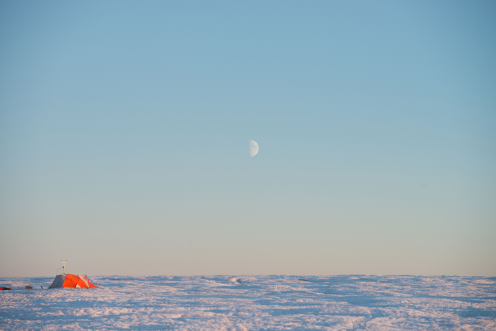
The view from the river toward our tents. (Photo by: Charlie Kershner).
Now that we’re back home, the process of data registration and processing begins. It’s not quite as much fun as collecting the data in such an amazing place, but we’re all excited to see what the data tells us about the dynamic processes in the ablation zone of the Greenland Ice Sheet.
If you want to see what LIDAR data looks like for yourself, check out plas.io or speck.ly, and interact with some sample data in a web browser. Also, GRiD and OpenTopo are two places with lots of LIDAR data from all over the world that you can download and explore.