Every year, a group of scientists affiliated with the Global Carbon Project give Earth something like an annual checkup. Among the key questions they address: how much carbon is stored in the atmosphere, the ocean, and the land? And how much of that carbon has moved from one reservoir to another through fossil fuel burning, deforestation, reforestation, and uptake by the ocean each year?
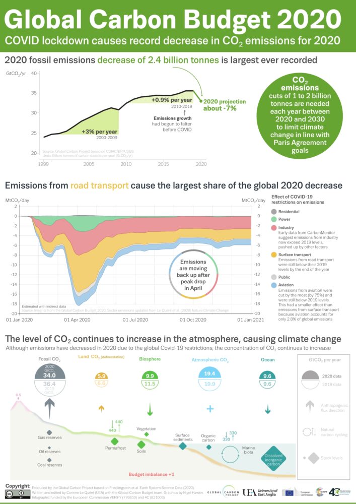
All of the latest findings—including the data for 2020, a year like few others—are available here, including links to dozens of interesting charts and a peer-reviewed science paper. Ben Poulter, a NASA scientist and member of the Global Carbon Project team, summarized the findings this way: “The economic effects of COVID-19 caused fossil fuel emissions to decrease by 7 percent in 2020, but we continued to see atmospheric CO2 concentrations increase, by 2.5 ppm, or about 5.3 PgC. This means that the remaining carbon budget to avoid 1.5 or 2 degrees warming continues to shrink, and that we need to continue to monitor the land, ocean, and atmosphere to understand where fossil fuel CO2 ends up.”
Below are 10 key findings from the most recent report. (Note: the Global Carbon Project team synthesizes a broad range of data, some of which requires time-consuming processing, quality-control, and analysis. While they do report some 2020 numbers, the most recent full year of data available for others is 2019.)


The Global Carbon Budget is produced by more than 80 researchers working from universities and research institutions in 15 countries. Observations from several NASA satellites, sensors, aircraft, and models were among the sources of information used to formulate the 2020 budget. Sources of information supported by NASA included: the MODIS sensors on Aqua and Terra satellites, the Global Fire Emissions Database (GFED), the LPJ land surface carbon exchange model, Landsat, the LUHv2 land-cover change model, the CASA land surface carbon exchange model, ODIAC fossil fuel emissions data, the MERRA-2 reanalysis, the Cooperative Global Atmospheric Data Integration Project, and OCO-2.
If you follow science news, this will probably sound familiar.
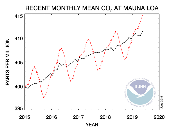
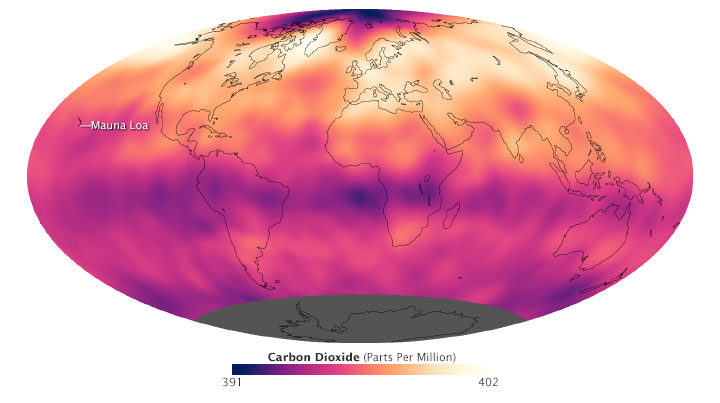
In May 2019, when atmospheric carbon dioxide reached its yearly peak, it set a record. The May average concentration of the greenhouse gas was 414.7 parts per million (ppm), as observed at NOAA’s Mauna Loa Atmospheric Baseline Observatory in Hawaii. That was the highest seasonal peak in 61 years, and the seventh consecutive year with a steep increase, according to NOAA and the Scripps Institution of Oceanography.
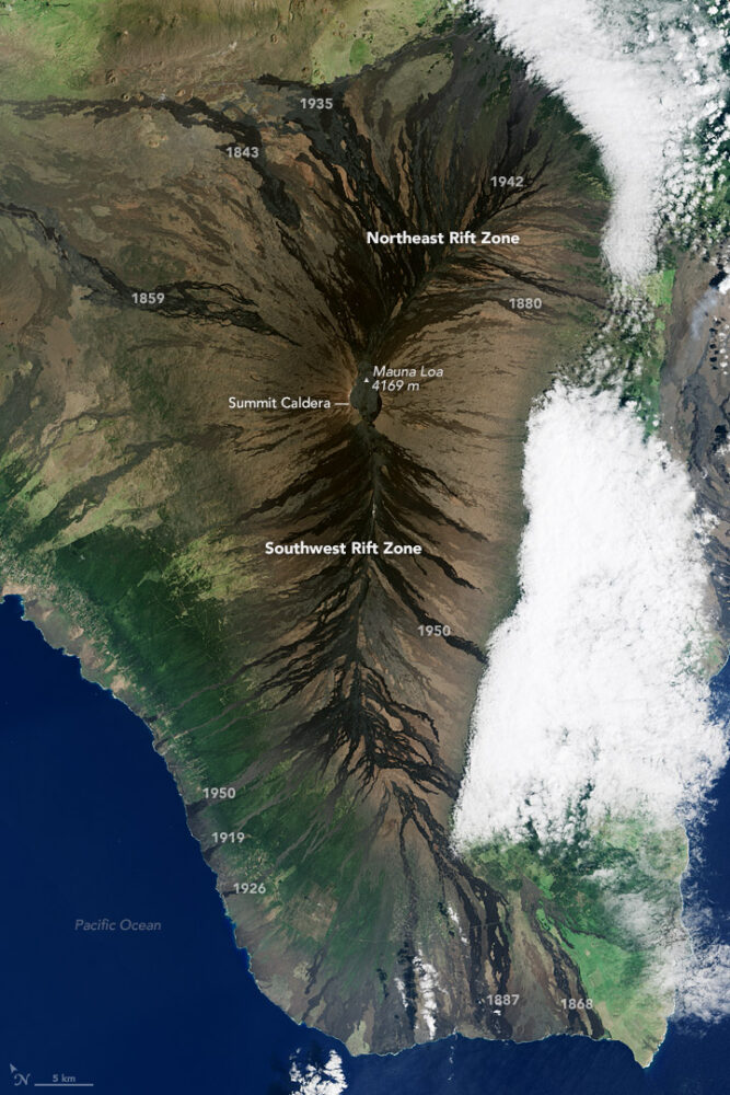
The Mauna Loa Observatory has been measuring carbon dioxide since 1958. The remote location (high on a volcano) and scarce vegetation make it a good place to monitor carbon dioxide because it does not have much interference from local sources of the gas. (There are occasional volcanic emissions, but scientists can easily monitor and filter them out.) Mauna Loa is part of a globally distributed network of air sampling sites that measure how much carbon dioxide is in the atmosphere.
The broad consensus among climate scientists is that increasing concentrations of carbon dioxide in the atmosphere are causing temperatures to warm, sea levels to rise, oceans to grow more acidic, and rainstorms, droughts, floods and fires to become more severe. Here are six less widely known but interesting things to know about carbon dioxide.
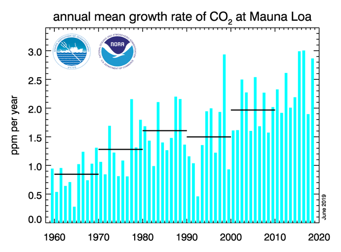
For decades, carbon dioxide concentrations have been increasing every year. In the 1960s, Mauna Loa saw annual increases around 0.8 ppm per year. By the 1980s and 1990s, the growth rate was up to 1.5 ppm year. Now it is above 2 ppm per year. There is “abundant and conclusive evidence” that the acceleration is caused by increased emissions, according to Pieter Tans, senior scientist with NOAA’s Global Monitoring Division.
To understand carbon dioxide variations prior to 1958, scientists rely on ice cores. Researchers have drilled deep into icepack in Antarctica and Greenland and taken samples of ice that are thousands of years old. That old ice contains trapped air bubbles that make it possible for scientists to reconstruct past carbon dioxide levels. The video below, produced by NOAA, illustrates this data set in beautiful detail. Notice how the variations and seasonal “noise” in the observations at short time scales fade away as you look at longer time scales.
Satellite observations show carbon dioxide in the air can be somewhat patchy, with high concentrations in some places and lower concentrations in others. For instance, the map below shows carbon dioxide levels for May 2013 in the mid-troposphere, the part of the atmosphere where most weather occurs. At the time there was more carbon dioxide in the northern hemisphere because crops, grasses, and trees hadn’t greened up yet and absorbed some of the gas. The transport and distribution of CO2 throughout the atmosphere is controlled by the jet stream, large weather systems, and other large-scale atmospheric circulations. This patchiness has raised interesting questions about how carbon dioxide is transported from one part of the atmosphere to another—both horizontally and vertically.
In this animation from NASA’s Scientific Visualization Studio, big plumes of carbon dioxide stream from cities in North America, Asia, and Europe. They also rise from areas with active crop fires or wildfires. Yet these plumes quickly get mixed as they rise and encounter high-altitude winds. In the visualization, reds and yellows show regions of higher than average CO2, while blues show regions lower than average. The pulsing of the data is caused by the day/night cycle of plant photosynthesis at the ground. This view highlights carbon dioxide emissions from crop fires in South America and Africa. The carbon dioxide can be transported over long distances, but notice how mountains can block the flow of the gas.
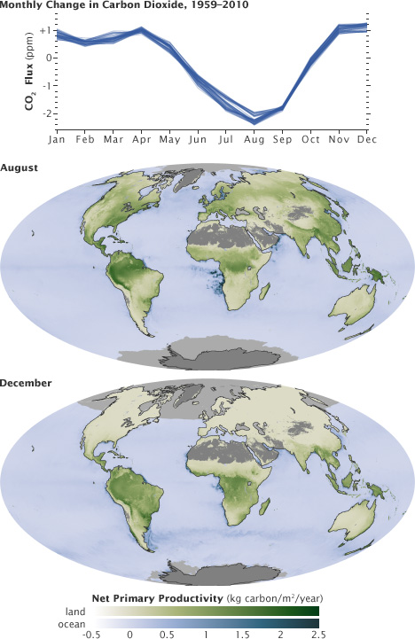
You’ll notice that there is a distinct sawtooth pattern in charts that show how carbon dioxide is changing over time. There are peaks and dips in carbon dioxide caused by seasonal changes in vegetation. Plants, trees, and crops absorb carbon dioxide, so seasons with more vegetation have lower levels of the gas. Carbon dioxide concentrations typically peak in April and May because decomposing leaves in forests in the Northern Hemisphere (particularly Canada and Russia) have been adding carbon dioxide to the air all winter, while new leaves have not yet sprouted and absorbed much of the gas. In the chart and maps below, the ebb and flow of the carbon cycle is visible by comparing the monthly changes in carbon dioxide with the globe’s net primary productivity, a measure of how much carbon dioxide vegetation consume during photosynthesis minus the amount they release during respiration. Notice that carbon dioxide dips in Northern Hemisphere summer.
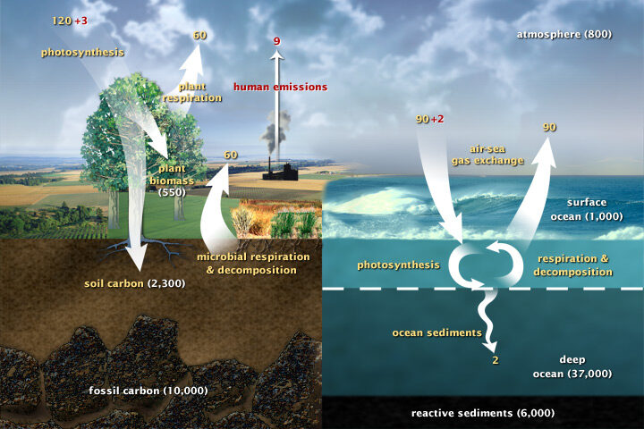
Most of Earth’s carbon—about 65,500 billion metric tons—is stored in rocks. The rest resides in the ocean, atmosphere, plants, soil, and fossil fuels. Carbon flows between each reservoir in the carbon cycle, which has slow and fast components. Any change in the cycle that shifts carbon out of one reservoir puts more carbon into other reservoirs. Any changes that put more carbon gases into the atmosphere result in warmer air temperatures. That’s why burning fossil fuels or wildfires are not the only factors determining what happens with atmospheric carbon dioxide. Things like the activity of phytoplankton, the health of the world’s forests, and the ways we change the landscapes through farming or building can play critical roles as well. Read more about the carbon cycle here.
A boatload of scientists headed out to sea this week. Actually, two boatloads. Both the R/V Salley Ride and the R/V Roger Revelle are taking part in a mission called Export Processes in the Ocean from Remote Sensing (EXPORTS).
Their plan: track what happens to carbon as it sinks from the well-lit surface of the ocean down to the dimmer “twilight zone” (between 650 feet and 3300 feet below the surface) using floats, gliders, and other scientific equipment. Then they’ll try to do the same thing using satellites.
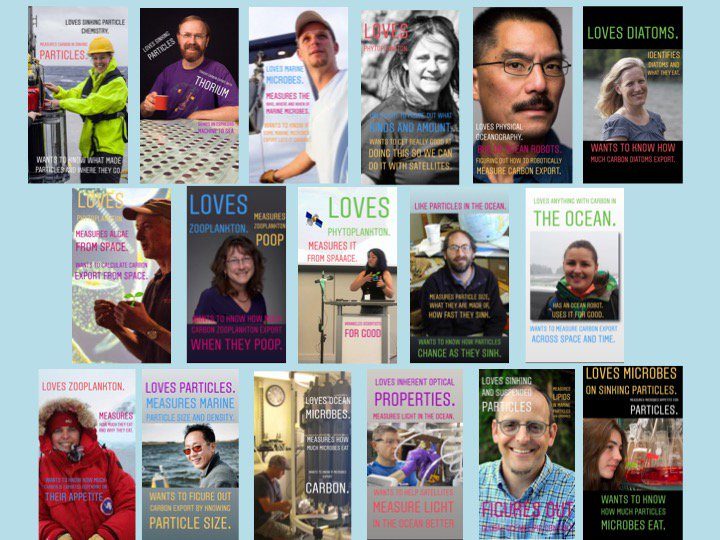
To help spread the word about the scientific work the team will be doing, oceanographer and blogger Kim Martini put together a fun set of #sciencetradingcards that people have been passing around on social media. Maybe she’ll roll out phytoplankton and zooplankton trading cards next?
Read more about the project from the mission website, a NASA Goddard press release, and the videos below. See a sample of the trading cards at the bottom of the page.
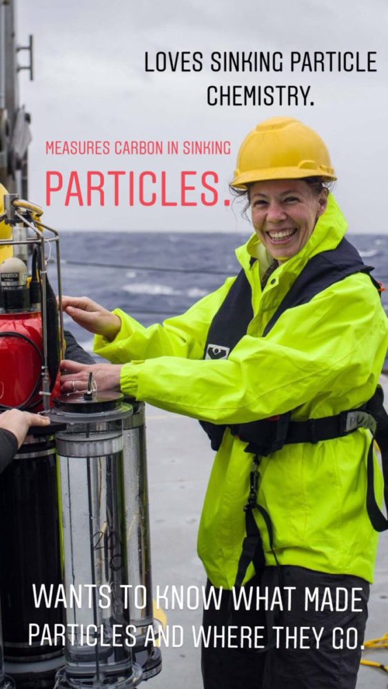
Project Title: Linking sinking particle chemistry and biology with changes in the magnitude and efficiency of carbon export into the deep ocean Project Lead: Margaret Estapa, Skidmore College
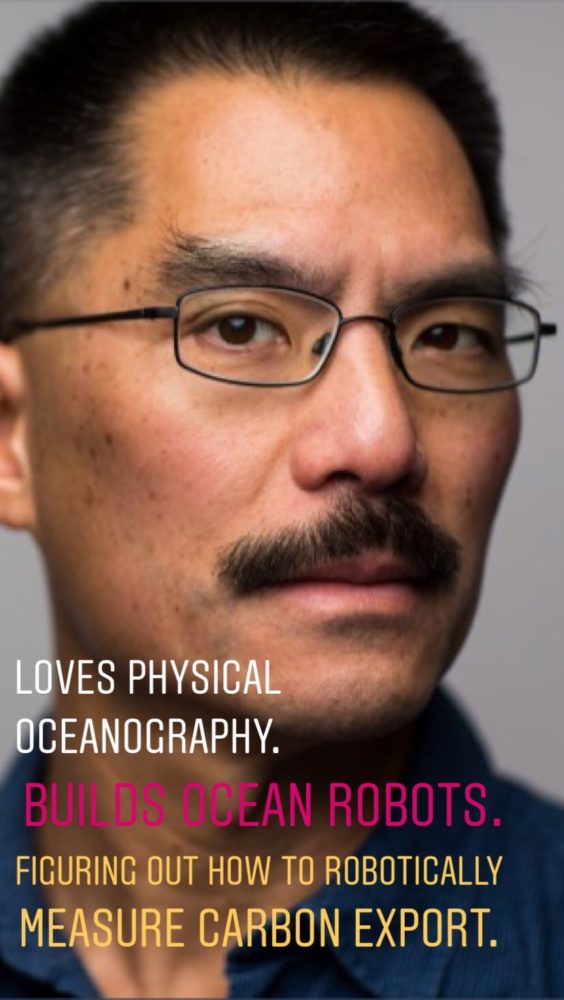
Project Title: Autonomous Investigation of Export Pathways from Hours to Seasons
Project Lead: Craig Lee – University of Washington
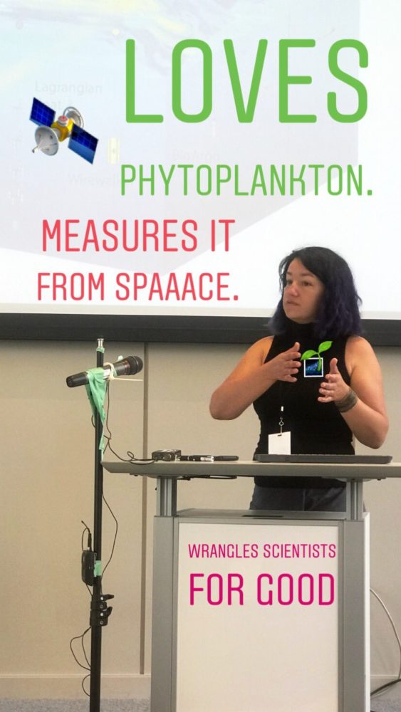
Ivona Cetinic – EXPORTS Project Scientist
NASA Goddard Space Flight Center/USRA
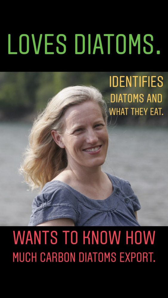
Project Title: Diatoms, Food Webs and Carbon Export – Leveraging NASA EXPORTS to Test the Role of Diatom Physiology in the Biological Carbon Pump Project Lead: Bethany Jenkins, The University of Rhode Island
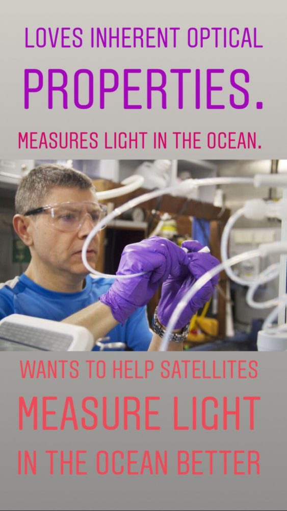
Project Title: In Situ Optics and Biogeochemistry in Support of EXPORTS Science Project Lead: Antonio Mannino, NASA Goddard Space Flight Center
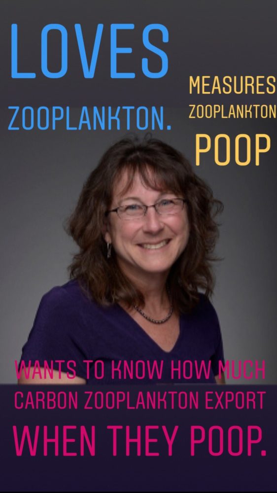
Project Title: Zooplankton-Mediated Export Pathways: Quantifying Fecal Pellet Export and Active Transport by Diel and Ontogenetic Vertical Migration in the North Pacific Project Lead: Deborah Steinberg, Virginia Institute of Marine Science
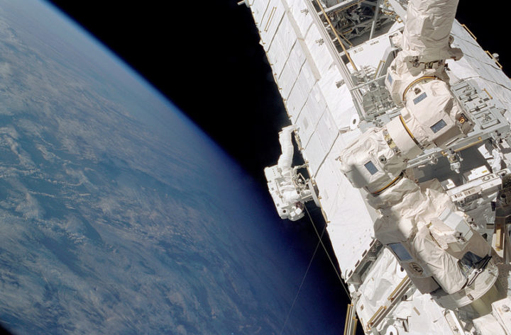
Piers Sellers during a spacewalk outside of the International Space Station. Credit: NASA
Astronaut and scientist Piers Sellers is no longer with us, but his words still resonate.
A posthumous plea from Sellers arrived in July 2018 in the form of an article in PNAS. The topic was one that he cared deeply about: building a better space-based system for observing and understanding the carbon cycle and its climate feedbacks.
As NASA’s Patrick Lynch reported, Sellers wrote the paper along with colleagues at NASA’s Jet Propulsion Laboratory and the University of Oklahoma. Work on the paper began in 2015, and Sellers continued working with his collaborators up until about six weeks before he died. They carried on the research and writing of the paper until its publication in July 2018.
The carbon cycle refers to the constant flow of carbon between rocks, water, the atmosphere, plants, soil, and fossil fuels. Climate change feedbacks—natural effects that may amplify or diminish the human emissions of greenhouse gases—are one of the most poorly understood aspects of climate science.
Here is how Sellers and colleagues characterized the current state of the carbon cycle in the PNAS article:
“It is quite remarkable and telling that human activity has significantly altered carbon cycling at the planetary scale. The atmospheric concentrations of carbon dioxide (CO2) and methane (CH4) have dramatically exceeded their envelope of the last several million years.”
They also explain in detail how we have altered the carbon cycle:
“The perturbation by humans occurs first and foremost through the transfer of carbon from geological reservoirs (fossil fuels) into the active land–atmosphere–ocean system and, secondarily, through the transfer of biotic carbon from forests, soils, and other terrestrial storage pools (e.g., industrial timber) into the atmosphere.”
Scientists understand the broad outlines of how this works relatively well. What worried Sellers was the potential curve balls the climate might throw at us with unanticipated feedbacks. They addressed some of the the challenges in understanding how climate change might affect concentrations of carbon dioxide and methane through feedbacks.
For carbon dioxide:
“While experimental studies consistently show increases in plant growth rates under elevated CO2 (termed carbon dioxide fertilization), the extrapolation of even the largest-scale experiments to ecosystem carbon storage is problematic, and some ecologists have argued that the physiological response could be eliminated entirely by restrictions due to limitation by nutrients or micronutrients. However, there is recent evidence from the atmosphere that suggests increasing CO2 enhances terrestrial carbon storage, leading to the continued increase in land uptake paralleling CO2 concentrations.”
As we detailed in a separate story, the situation is even more complicated for methane. Sellers and his colleagues explained some of the challenges in understanding the feedbacks that affect that potent greenhouse gas this way:
“Atmospheric methane is currently at three times its preindustrial levels, which is clearly driven by anthropogenic emissions, but equally clearly, some of the change is because of carbon-cycle–climate feedbacks. Atmospheric CH4 rose by about 1 percent per year in the 1970s and 1980s, plateaued in the 1990s, and resumed a steady rise after 2006. Why did the plateau occur? These trends in atmospheric methane concentration are not understood. They may be due to changes in climate: increases in temperature, shifts in the precipitation patterns, changes to wetlands, or proliferation in the carbon availability to methane-producing bacteria.”
The consequences of the gaps in understanding could be significant.
“Terrestrial tropical ecosystem feedbacks from the El Nino drove an ∼2-PgC increase in global CO2 emissions in 2015. If emissions excursions such as this become more frequent or persistent in the future, agreed-upon mitigation commitments could become ineffective in meeting climate stabilization targets. Earth system models disagree wildly about the magnitude and frequency of carbon–climate feedback events, and data to this point have been astonishingly ineffective at reducing this uncertainty.”
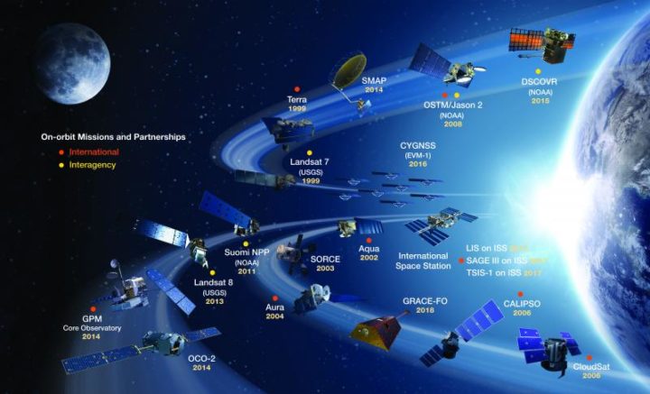
NASA’s current missions and partnership missions in orbit. Credit: NASA
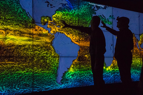
Sellers and his colleagues do offer a solution. It has much to do with satellites.
“Space-based observations provide the global coverage, spatial and temporal sampling, and suite of carbon cycle observations required to resolve net carbon fluxes into their component fluxes (photosynthesis, respiration, and biomass burning). These space-based data substantially reduce ambiguity about what is happening in the present and enable us to falsify models more effectively than previous datasets could, leading to more informed projections.”
