We have spent the last few weeks discussing the differences between inherent and apparent optical properties in the ocean and how we measure them. Now let’s take a moment to appreciate the information these data give us. I am sure many of you have seen satellite images of the ocean, hurricanes, etc. on the news and at other outlets. A lot of work goes into each and every one of those images and they can show remarkable things on a global scale that would be difficult to detect through fieldwork alone.
Below you will see a true color image of a phytoplankton bloom in the Barents Sea that was acquired on August 24, 2012 by NASA’s MODIS Aqua satellite . The Barents Sea is part of the Arctic Ocean and is located off the northern coasts of Norway and Russia. The word phytoplankton is Latin for plant (phyto) and to wander or drift (plankton). Phytoplankton can photosynthesize and produce energy from sunlight just like plants do on land. They also take up carbon dioxide and release oxygen like land plants. Phytoplankton are an important component of the food chain as other organisms such as zooplankton and fish use them as a food source. Additionally, they play an important role in the global carbon budget because they can use the carbon (CO2) that is absorbed by the ocean to make sugars.
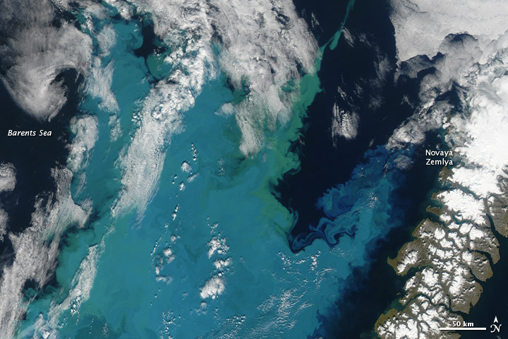
Barents Sea phytoplankton Bloom
There are many types of phytoplankton that bloom in the ocean including diatoms, dinoflagellates, and coccolithophores, just to name a few. You can learn more about different phytoplankton groups here. They all rely on specific nutrients, such as nitrogen (NO3, NO2, etc.), phosphorous (PO4, etc.) and trace metals (iron, magnesium, etc.). Phytoplankton blooms occur when many individuals, or cells, of one species are present in one region of a body of water (lake, estuary, open ocean), altering the color of the water. In the image above, the water is dominated by a species of coccolithophore. Coccolithophores are a type of phytoplankton that are covered with plates made of calcite called coccoliths. Calcite, or calcium carbonate, is white giving that creamy white look to the water. You can learn more about this coccolithophore bloom here.
This next image was recently featured on NASA’s OceanColor website. It was taken off the western coast of Africa where a current called the Benguela current flows northward bringing water from the South Atlantic and Indian Ocean. In this image from April 10, 2014 we can see a yellow discoloration in the water. I just learned that this area is prone to toxic hydrogen sulfide precipitation events that have been known to cause fish and other marine animal mortalities. Amazingly, these events have been captured using satellite imagery. However, the cause of this particular discoloration has not, as of this post, been determined. This is where fieldwork comes in! Still, it is very cool! Thanks to Norman Kuring at NASA Goddard for locating this feature.

Discoloration in the Benguela Current off the coast of Namibia
You can enjoy many other satellite images at NASA’s Visible Earth website.
References:
http://www.worldatlas.com/aatlas/infopage/barentssea.htm
http://earthobservatory.nasa.gov/Features/Phytoplankton/
http://www.bigelow.org/foodweb/microbe0.html
http://protozoa.uga.edu/portal/coccolithophores.html
http://oceancolor.gsfc.nasa.gov/
http://oceancurrents.rsmas.miami.edu/atlantic/benguela.html
http://oceancolor.gsfc.nasa.gov/cgi/image_archive.cgi?i=423
http://www.sciencedirect.com/science/article/pii/S0967063703001754
ACKNOWLEDGEMENTS: NASA’s Ocean Ecology Laboratory Field Support Group is participating in the US Repeat Hydrography, P16S field campaign under the auspices of the International Global Ocean Ship-Based Hydrographic Investigations Program (GO-SHIP). The US Climate Variability and Predictability Program (CLIVAR), NOAA and the NSF sponsor this campaign.

One of the greatest tools used by oceanographers today for measuring ocean processes is the CTD. CTD stands for Conductivity, Temperature and Depth. Conductivity is a measure of ocean salinity. The CTD is used to collect profile data in the ocean. The CTD is typically accompanied by a carousel, or rosette, of large bottles (Niskins) that can hold about 10 liters (2.6 U.S. gallons) of water. Some Niskins are large enough to hold 30 liters. These bottles have spring-loaded caps that can be triggered to close at specified depths. The CTD and other sensors, such as a chlorophyll fluorometer, and an Acoustic Doppler Current Profiler (ADCP) that measures current velocities, and other sensors can also be attached within the rosette package.
The whole package is connected to a very long cable and is mechanically lowered by a winch operator down through the water column, which is called the ‘downcast.’ During the downcast, information about salinity, temperature, depth and data from the other sensors are sent to a computer on board the ship. The computer is connected through the cable that is lowering the package. The downcast is halted once the package reaches close to the ocean floor. When the CTD is raised back to the surface, the ‘upcast’, each of the Niskin bottles is closed at assigned depths, collecting water as it travels back to the surface.
Once the Rosette package is back aboard the ship, the scientists are able to collect water from the bottles for their analyses. The parameters collected and analyzed during CLIVAR campaigns includes but are not limited to: salinity, oxygen, nutrients, chlorofluorocarbons (CFCs), dissolved inorganic carbon (DIC), total alkalinity, pH, dissolved organic carbon (DOC), helium, and tritium.
Certain compounds, such as some radionuclide (tritium, carbon-14, etc.) and CFCs, can be used as ‘tracers’. These tracers are used to follow ocean currents and calculate the age of water parcels. CFCs were prominently used in refrigerators and air conditioning units until the 1970s when they were banned over the concern of ozone depletion. You can learn more about the CFC tracer program here. Through the WOCE and CLIVAR programs CFC concentrations have been measured all over the world.
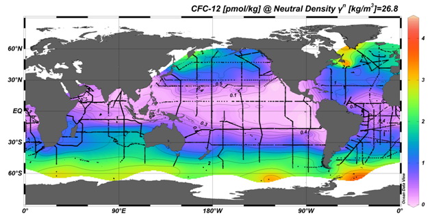
Map of global CFC measurements
http://www.pmel.noaa.gov/cfc/
The measurement of pH, total alkalinity and DIC are important for monitoring ocean acidification. Ocean acidification (OA) is the decrease in ocean pH as a result of an increase in carbon dioxide (CO2) absorption by seawater. OA is a prominent concern in today’s world. CO2 is pumped into the atmosphere from everyday human activities, such as emissions from vehicles and industrial pollution. Each year approximately 25% of the CO2 pumped into the atmosphere is absorbed by the ocean. Although plants can use CO2 for photosynthesis, the increase also has negative implications. As the amount of CO2 absorbed by the increases, the pH is expected to continue decreasing.
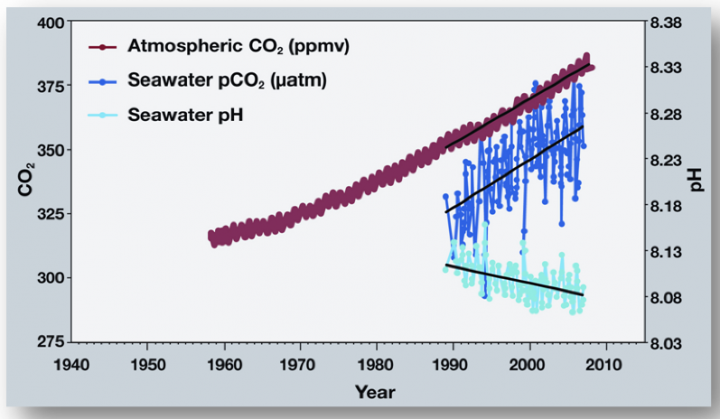
pH time series
http://www.pmel.noaa.gov/co2/story/OA+Observations+and+Data
The pH of the ocean directly affects organisms that form calcium carbonate shells or structures, like corals, oysters, clams and sea urchins. An acidic environment causes the calcium carbonate to dissolve and makes it more difficult for the organisms to make their calcium carbonate skeletons. Therefore, it is important that programs like CLIVAR are monitoring global CO2 concentrations (part of the DIC pool), total alkalinity (the ability for the ocean to neutralize acids) and pH. We know that decreases in ocean pH can negatively impact marine organisms. You can see more about the effect of ocean acidification or marine organisms here.
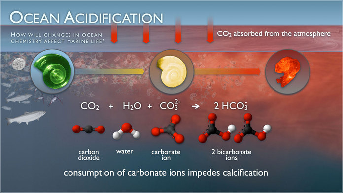
Ocean Acidification
http://www.pmel.noaa.gov/co2/story/What+is+Ocean+Acidification%3F
As I was conducting some research for this blog post I came across this article that was posted at the Earth Observatory in 2008 about the global carbon budget. I thought it was appropriate to bring it back here.
Earth Observatory article from 2008
References:
http://www.whoi.edu/home/oceanus_images/ries/calcification.html
http://www.pmel.noaa.gov/co2/story/What+is+Ocean+Acidification%3F
http://water.me.vccs.edu/exam_prep/alkalinity.html
http://earthobservatory.nasa.gov/Features/OceanCarbon/
http://rspb.royalsocietypublishing.org/content/275/1644/1767.full
ACKNOWLEDGEMENTS: NASA’s Ocean Ecology Laboratory Field Support Group is participating in the US Repeat Hydrography, P16S field campaign under the auspices of the International Global Ocean Ship-Based Hydrographic Investigations Program (GO-SHIP). The US Climate Variability and Predictability Program (CLIVAR), NOAA and the NSF sponsor this campaign.
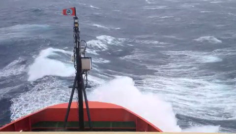
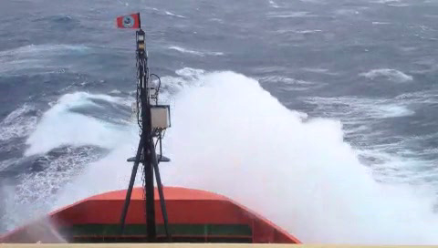
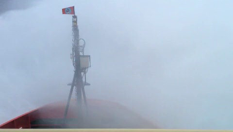
The NASA FSG folks and the rest of the science crew on the US Repeat Hydrography P16S field campaign have experienced some weather delays, which can be expected when working the Southern Ocean close in time to the Southern Hemisphere winter. They encountered 45-knot winds (~51 miles per hour) sitting on top of their planned sampling area at around 60 degrees South latitude. For the safety of all they could not conduct science under those conditions. So they traveled ~200 miles north to escape the weather and then returned southward once the weather had settled. Below you will see some freeze frame clips from the movie Joaquin Chaves captured showing the large swells and the dramatic gray skies of the Southern Ocean. The movie was recorded through the porthole, safe inside the ship.

Stormy weather 1

Stormy weather 2
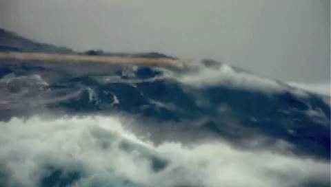
Stormy weather 3
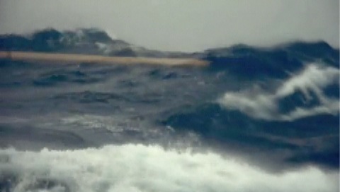
Stormy weather 4
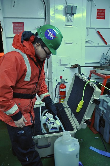
In spite of the rough weather, the FSG fellows have taken advantage of some calmer days to deploy a radiometer. A radiometer measures apparent optical properties or AOPs. You might recall from Blog #2 that we discussed Inherent Optical Properties or IOPS that characterize the absorption and scattering (reflecting) of light by dissolved and particulate materials in the water. The measurement of IOPs can be done at any time day or night. AOPs on the other hand must be measured during the daytime, preferable when there are clear skies and the sun is directly overhead. AOPs describe how the light is entering and exiting the water column. Remember that sunlight contains a whole spectrum of colors that are determined by their wavelength. We see what is called the “visible spectrum” like what is in the image below.
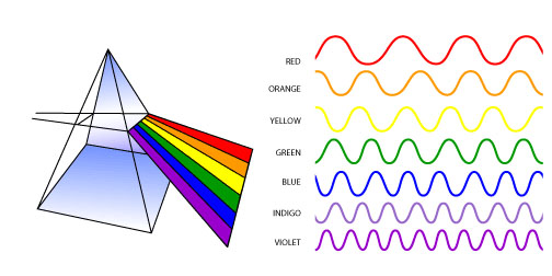
As the sunlight penetrates the water column, some of the light is absorbed, some is scattered (reflected) backward toward the sky and the rest is scattered forward into the depths of the ocean. Water itself absorbs most of the red light, so we never really see a red ocean (unless there is something unusual in the water).
The character of the light that is reflected back out of the water can be different than what went in. More specifically, the wavelengths or colors that are reflected back out are the colors that were not absorbed or scattered forward. Think about when you are at the beach, say Ocean City, MD or Rehoboth Beach, Delaware. The water typically looks brown or green, right? This is because particles, including both algae and sediment (and water), are absorbing all of the blue and red light, and the leftover colors of brown and green are reflected back out. Conversely, for those of you who have seen blue water in places like the Caribbean or around Bermuda, the circumstances are different. There are very few particles or phytoplankton in the water to absorb the blue light like in the coastal water. Therefore, that blue color is reflected back out , which is why the water looks so blue and pretty. A radiometer that the FSG is deploying on this field campaign measures the colors and amount of the light entering and exiting the water column. The radiometer is hand deployed and, I can tell you, it’s a lot of work!
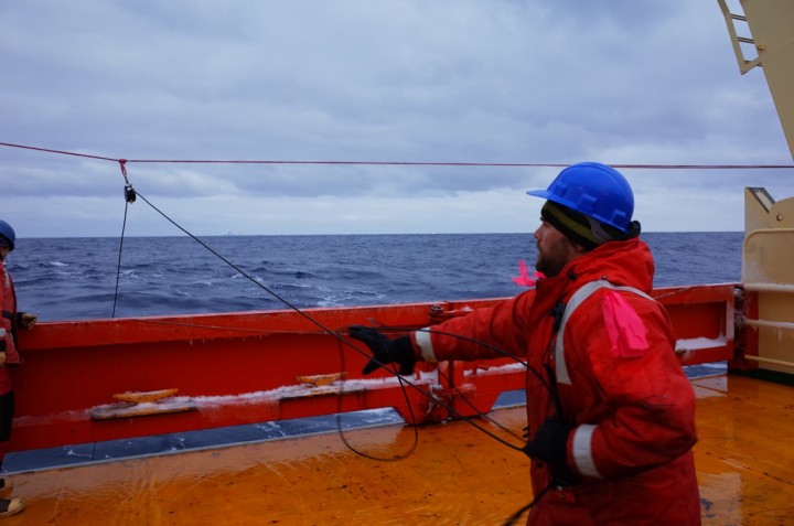
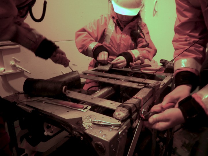
Joaquin and Scott preparing to deploy the radiometer
Photo credit: Isabella Rosso
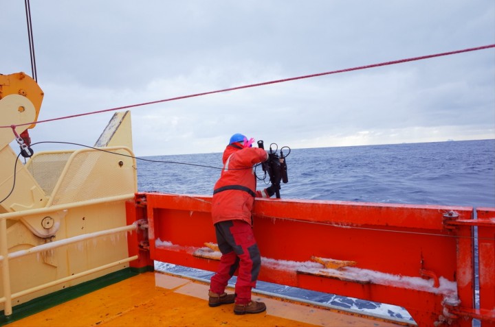
Dropping the radiometer into the water
Photo credit: Scott Freeman
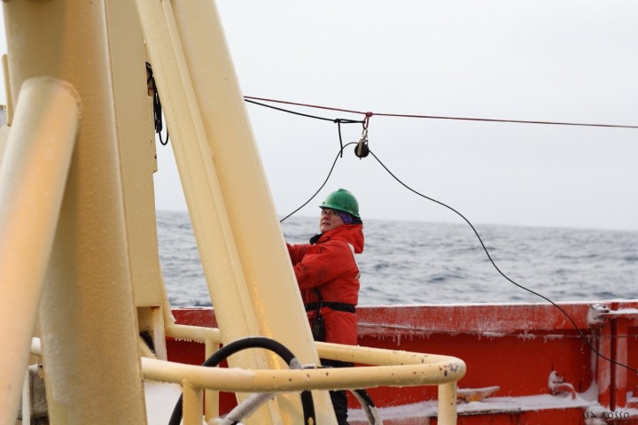
Joaquin guiding the cable; Photo credit Isabella Rosso
Mike pulling the radiometer back to the surface
Satellite instruments, such as SeaWiFS (no longer operational) and MODIS-Aqua (operational) measures this light just like the radiometer so that we can get beautiful images that you can see below.
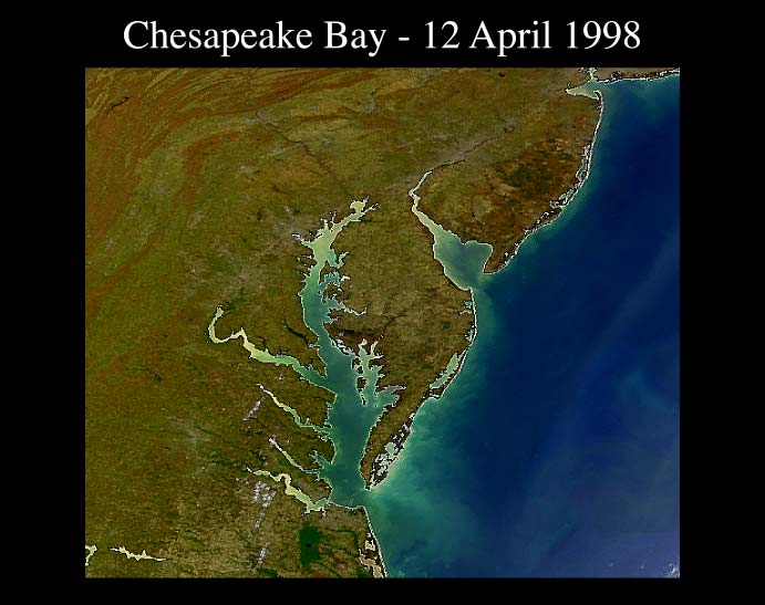
True color image of Chesapeake Bay
http://oceancolor.gsfc.nasa.gov
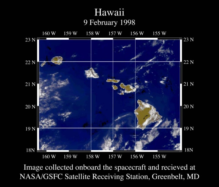
True color image of Hawaii
http://oceancolor.gsfc.nasa.gov
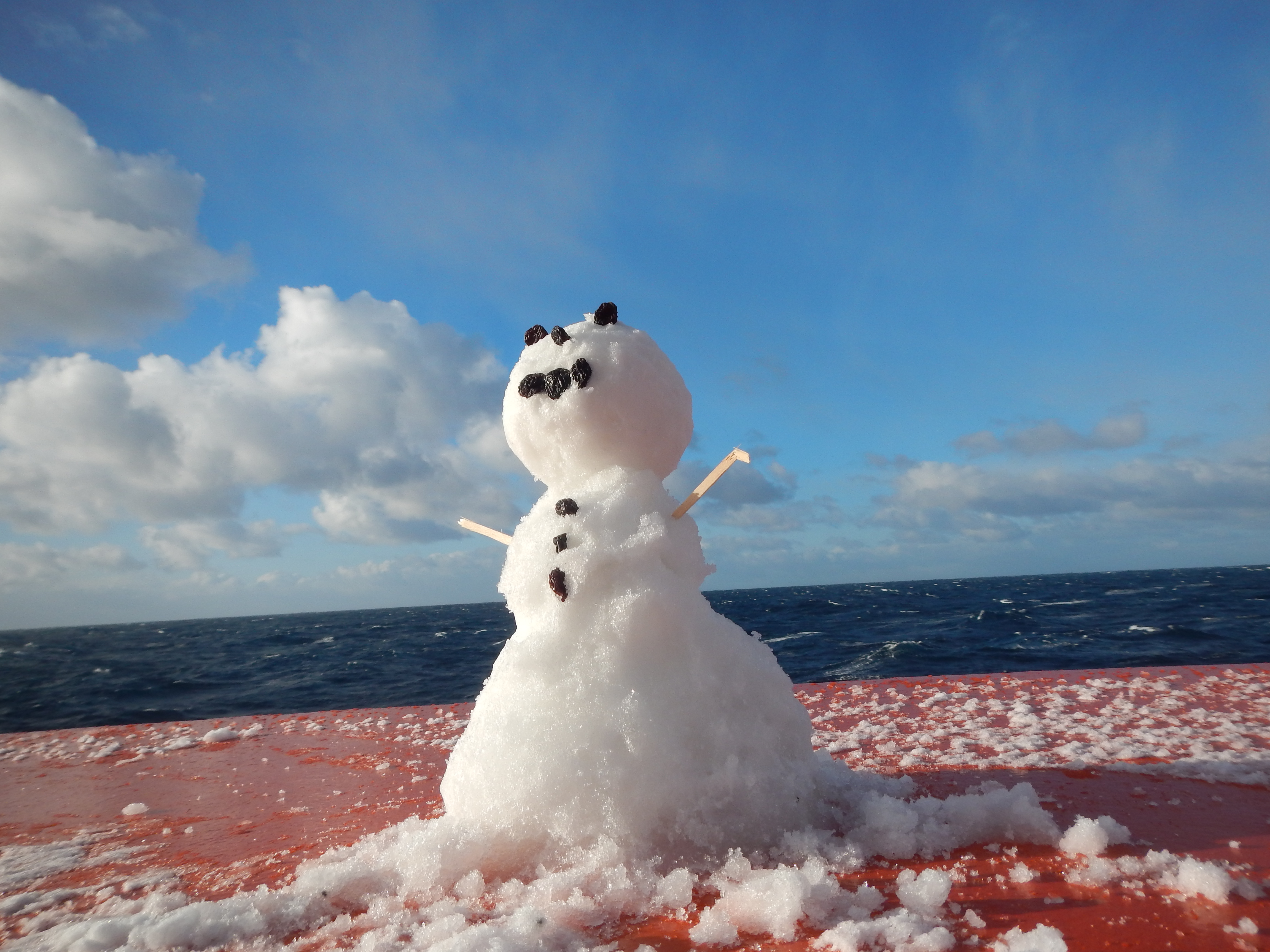
Our FSG fellas are working very hard during this field campaign. But every now and then you need to have a little fun. Mike Novak sent this picture of a snowman that was built on the bow of the ship. I think the eyes, nose, and buttons are raisins.
References:
http://ushydro.ucsd.edu/p16s-weekly-reports/
http://www.oceanopticsbook.info/
http://oceancolor.gsfc.nasa.gov
ACKNOWLEDGEMENTS: NASA’s Ocean Ecology Laboratory Field Support Group is participating in the US Repeat Hydrography, P16S field campaign under the auspices of the International Global Ocean Ship-Based Hydrographic Investigations Program (GO-SHIP). The US Climate Variability and Predictability Program (CLIVAR), NOAA and the NSF sponsor this campaign.
As many of you probably heard, there was an 8.2-magnitude earthquake off the coast of Northern Chile on Tuesday night. As with any earthquake around a coastal region or on the ocean floor, there is great concern about the formation of a tsunami. A Tsunami is series of waves with a very large wavelength. Think of a series of waves hitting a beach. The distance between each wave hitting the shore is the wavelength. Now picture a wavelength that is 100s of miles long! Because the wavelengths are so long, the waves travel at very high speeds, around 600 miles per hour, in the deep ocean. This is the speed at which a commercial jet plane travels! However, the wave height (the height from the base of the wave at the water line to the top of the wave) is very small, maybe a few feet tall. As you can imagine, a boat or ship in the open ocean wouldn’t even notice such a tiny wave.
Below is a screen shot from a CNN video report about the earthquake. In this video you can see how the waves propagate out from the source of the earthquake out into the ocean (red arrow).

Wave propagation
http://www.cnn.com/2014/04/01/world/americas/chile-earthquake/
The story changes, however, when the depth of the ocean decreases, such as when approaching land. All of that energy in that fast wave gets slowed down and subsequently the height of the wave gets bigger, and sea level near shore can rise at least 50 feet! Thankfully, our colleagues are out of harms way from tsunamis because they are in the middle of the deep, open ocean.
The ship and its inhabitants ARE, however, subject to waves that are created by storms and strong winds. Joaquin made a video of the wave action that you can see below. Here are some freeze frame ‘action shots’ from the video.
https://www.youtube.com/watch?v=cBTORY0aalE&feature=youtu.be
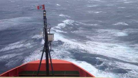
Stage 1
Stage 2
Stage 3
Stage 4
And, lastly, I thought it would be good to show some pictures of how cold it is that far south and how challenging it can be to work outside on deck in the cold. In this picture you can see icicles hanging off the ship during recovery of an IOP package deployment.
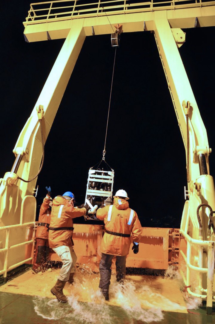
Water intrusion during recovery of the IOP package
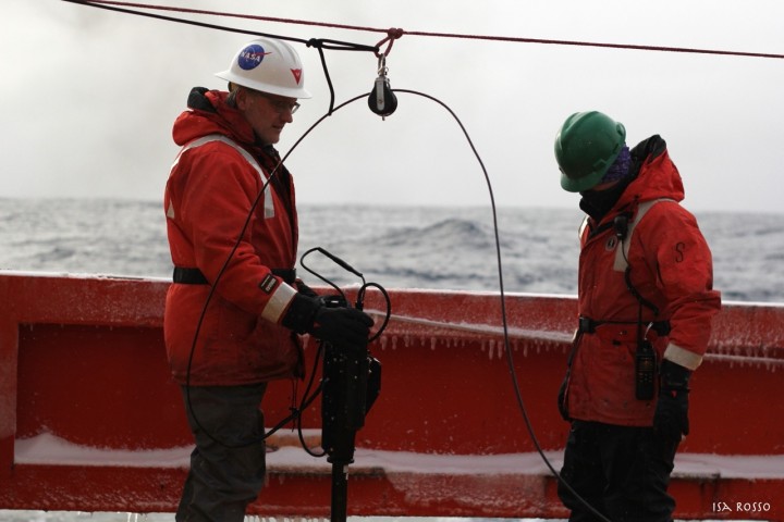
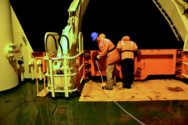
Mike and Scott are having a conversation as they wait for the IOP package to return to the surface of the ocean. I wonder what they are talking about???

A very intense conversation ensues while waiting for the IOP package to return to the ocean surface
You can watch an entire IOP deployment below.
Lastly, when working so close to the continent of Antarctica, there must be a sighting of an iceberg.

Iceberg!
Sources:
http://www.nws.noaa.gov/om/brochures/tsunami.htm
http://www.cnn.com/2014/04/01/world/americas/chile-earthquake/
At approximately 60° South and 174° East the FSG members sampled their first official station of the field campaign. The solid red line in the map below denotes the current ship track (as of March 27th). The ship has not yet reached the P16S line that begins at 150° West (the blue circles on the map below).

The FSG will deploy an IOP package at one station each day. The FSG IOP package is an assemblage of instruments that collect data for temperature, salinity, depth, absorption of particles and dissolved components, and particle scattering. The instruments are contained within a metal ‘cage’ that is lowered on a wire to a chosen depth in the water column. The data collected by the instruments are saved to a type of hard drive located within the cage. Before the cage can be deployed, weight must be added so that it can sink.
Adding weight to the IOP cage
Here, the cage with all of the instruments is being lifted off the deck of the ship and lowered into the water.
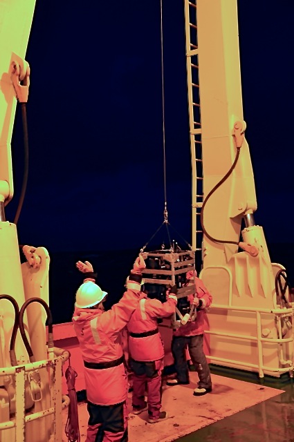
Deploying the IOP package off the side of the ship
And, sometimes, King Neptune decides to send a wave your way. But that is why we wear our safety gear!
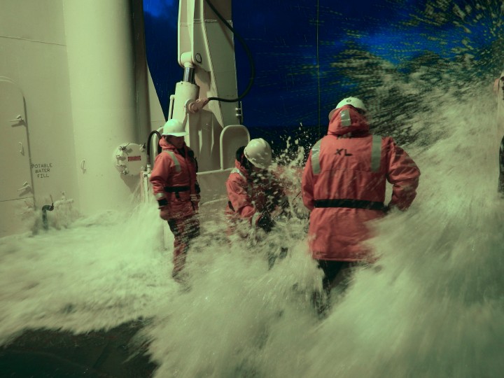
Scott catching a wave-It’s all part of the job
The FSG also collects surface water samples in conjunction with the IOP package deployment. A weighted tube is lowered over the side of the ship, and a large peristaltic pump gently transfers seawater to a large container (carboy).
Lowering tubing over the side of the ship to collect surface water
Joaquin filling a carboy with surface water pumped off the side of the ship
The water is filtered and processed back in the laboratory on the ship.
Now, let’s take a moment to understand the significance and importance of hydrographic field campaigns. Oceanic and atmospheric processes are tightly coupled. Temperature and freshwater fluxes between the ocean and atmosphere are in control of climate variability. A good example of this strong ocean-atmosphere relationship is El Nino Southern Oscillation or ENSO. During an El Nino event, the temperature structure of the equatorial Pacific Ocean is disrupted. The central equatorial Pacific Ocean becomes warmer than normal affecting tropical rainfall in Indonesia and global weather patterns. The objective of the Climate Variability and Predictability of the ocean-atmosphere system, or CLIVAR, program is to understand this dynamic coupling and model future ocean-atmosphere variability by collecting and analyzing ship-based global observations. The International CLIVAR program is a continuation of its predecessors: the Tropical-Ocean Global Atmosphere (TOGA) and the World Ocean Circulation Experiment (WOCE). The TOGA program was formed in 1985 to study the relationship between the tropical ocean and the global atmosphere with the ultimate goal of predicting variability on various time scales. The WOCE program began in 1990 with the objective to study global ocean circulation and its relationship to the global climate system over long time scales using global observations. The US-CLIVAR program contributes to the international program as well as the World Climate Research Program. You can learn more about the US-CLIVAR program here.
Image of global data from www.ewoce.org
