By Walt Meier
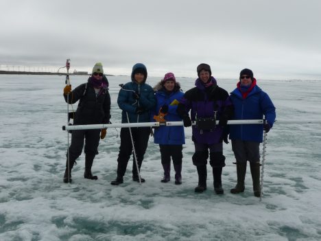
The Red Team on sea ice.
May 28, 2016 – This morning we did our first modeling exercise. We started simply, modeling the ice’s thickness as the balance between ice growth and ice melt. Ice grows during the winter and melts during the summer. But from this simple start, a lot can be gleaned. The growth and melt rates are influenced by many factors – the amount of solar energy onto the ice, the amount of energy lost from the surface, the heat from the ocean below. We used a simple model to adjust these parameters to see how the thickness responded. Even such a simple model can demonstrate how the sea ice responds to climate change. For example, just a slightly darker surface (e.g., due to more melt ponds during the summer) results in a thinner ice cover because there is more melt.
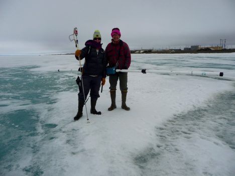
Two members of the Red Team holding the electromagnetic induction instrument to measure sea ice thickness.
In the afternoon, my group’s activity for the day was ice thickness measurements, led by Jackie Richter-Menge of the U.S. Army Cold Regions Research and Engineering Laboratory in New Hampshire. There were two methods we were shown how to use – drilling with an ice auger (a boring tool) and measuring thickness directly, as we did the day before, and using an electromagnetic (EM) induction instrument. The EM creates a magnetic field that is differently affected by the ice and water. The modification of the field indicates the thickness of the ice. The EM looks like a long pole with a box about the size of a car battery in the middle. You carry the box with a harness around your shoulder and the poles sticking out to each side. You need to hold the pole parallel relative to the ground. Working with it looks rather like a high-wire walker with a balance pole. Unfortunately, the EM instrument was not working, so we couldn’t collect any data, though we took turns carrying it to get an appreciation of what it’s like to use it. It’s just heavy enough and awkward enough to be a challenge, but when it works, it can provide a nice transect of thickness estimates and it’s quicker and easier than drilling holes.
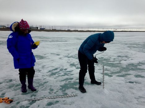
Two members of the Red team drilling with an ice auger.
Without the EM functioning, we had to rely on the ice auger. This is the most accurate way to measure sea ice thickness…or is it? Drilling a hole and using a tape measure is the most direct way to measure thickness and it is indeed most accurate – but only at that point. The ice is tremendously variable. As we saw during our morphology activity, thick 5 meter (16.4 feet) ice can be right next to first-year ice of 1 meter (3.3 feet) or less thickness. You could drill a hole and make the most accurate measurement possible, but it may be totally unrepresentative of the surrounding ice. This can be addressed to some degree by taking several measurements, but you can only cover so much area during a given expedition. It’s just not possible to cover 25-50 km model and satellite observation grid cells in a reasonable of time.
We set out a 200 meter (656 feet) line, drilling holes every 25 meters (82 feet). We also used a snow probe (a long stick you push down through the snow) to measure snow depth every 5 meters (16.4 feet). Part of the trick of doing these measurements is to make sure the observer doesn’t interfere with the measurement. So you don’t want to be making footprints where you measure, because you compress the ice. We set up the convention of walking on the left and measuring on the right. It sounds simple enough, but if you’re not always mindful of that, it’s easy to step over the line.
With our work finished, we ended the day in the traditional way for the Memorial Day weekend: with a BBQ! We had the traditional meal of hamburgers, hot dogs…and reindeer sausages. Along a number of delicious potluck sides brought over by the other huts, it was a great meal. We relaxed and enjoyed good food and good conversation while recounting our day’s adventures and discussing our research.
By Walt Meier
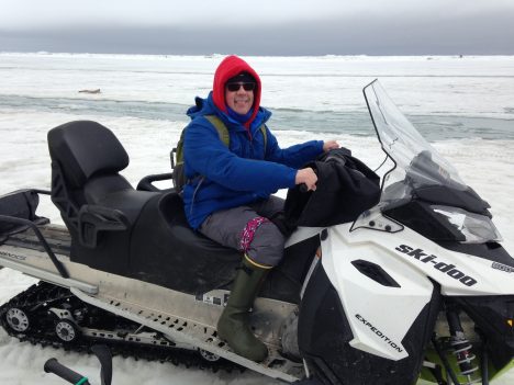
Walt Meier on a snowmobile.
May 27, afternoon – After our morning orientation and introduction sessions, I headed out onto the ice for the first time. We were split into four teams; each team will rotate through a different activity every day with each activity being led by one or two experts that will serve as our guide. I was assigned to the Red Team. Our activity for the day was sea ice morphology, or studying the forms of sea ice, and it was led by Chris Polashenski at the U.S. Army Cold Regions Research and Engineering Lab and Andy Mahoney at the University of Alaska, Fairbanks. All the other activities were being conducted within a short walk of the beach, but in order to see different types of ice, we needed to roam farther. This meant using snowmobile. After getting comfortable on the machines, we headed out. Our first stop was on a first-year ice floe, or is ice that has grown since the previous summer. This type of ice is generally thinner than multi-year ice (ice that has survived at least one summer melt season) and its thickness is largely controlled by the air temperature during the winter (though how much snow falls is important too). Colder temperatures mean more ice growth and thicker ice at the end of winter. We measured the thickness by drilling a hole through the ice using an auger. Then we dropped down a measuring tape. The tape has a folding metal bar at the end that catches the ice at the bottom of the hole; the tape is pulled taut and the thickness is read off the tape.
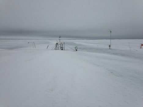
An ice mass balance station in Barrow, AK.
According to Chris and Andy, first-year ice in the area normally should be about 1.5 meters (5 feet) thick. We measured only 0.75 m. That means it’s been a very warm winter around here. But that is nothing new; in recent years, warm winters have become the norm as indicated by thickness measurements. For the past several years, Andy has been installing a sea ice mass balance station on the ice, automatically taking thickness readings every 15 minutes through the winter. The data is available online here.
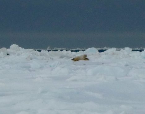
A polar bear in the distance.
Next we head further north, past Point Barrow, the northernmost land in the U.S., toward the fast ice edge. On the way, we spotted two polar bears in the distance. Polar bears are not an uncommon sight. They usually hang out near the ice edge hunting seals, though they sometimes wander into town, which can be a problem. At this time of year they are attracted by the whale carcasses that the native populations pull onto the ice as part of their traditional whale hunts. The bears were distant and barely visible, but it was quite exciting to see a bear. Polar bears can be dangerous and during all of our activities on the ice, we will have a polar bear spotter –a trained local resident carrying a shotgun – with us at all times.
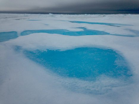
We left the polar bears to their business and rode further out to a multi-year ice floe that was more than 5 meters (16.4 feet) thick. We attempted to measure the thickness, but we didn’t break through the bottom of the ice at our auger’s (boring tool) maximum 5-meter length. To my untrained eye, the multiyear ice didn’t really look much different than first year. But with careful viewing, one could see an elevation change compared to the first-year ice. It wasn’t a lot, but a just little more elevation on the surface that floats above the ocean translates into much thicker ice because roughly 90 percent of the ice thickness lies beneath the surface of the waters. So a 5-meter thick floe of sea ice rises only about 50 cm (20 inches) above the waterline. The most distinguishing characteristic, at least at this time of year, are the brilliant blue melt ponds that form on the surface. As the snow melts, the melt water will accumulate in depressions in the ice, pooling into ponds. The crystal clear water on top of the pure multi-year ice produces a distinctive turquoise color reminiscent of the water around a tropical island. Melt ponds are very important because they absorb much more solar energy than the surrounding ice, which accelerates the melting process. But to be honest, when seeing a pond in person, the first thought one has is how pretty they are.
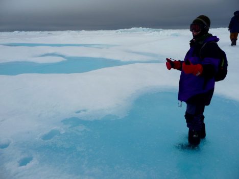
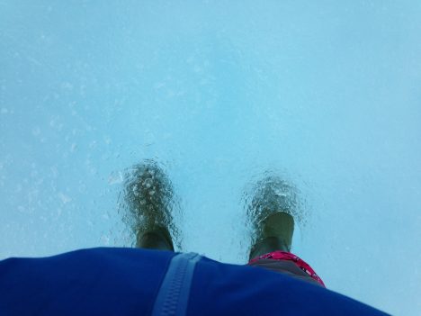
Walt, standing on a melt pond.
Just a few meters away, back on first-year ice, was another melt pond. But this had a much darker color due to the thinner and flatter ice. The water was also somewhat salty because first-year ice still retains some salt. The salt gets flushed out of the multiyear ice, so the blue ponds on the multiyear ice are fresh water suitable for drinking. We tried some and it was quite refreshing – ice cold!
Next, we headed over to a large piece of ridged ice. Ice ridges form due to ice floes being piled into each other due to winds or waves. The fast ice does not move, but the drifting ice beyond does and when the winds blow toward the land, the drifting ice collides with the fast ice, forming mountains of ice. The one we investigated was around 5 meters (16.4 feet) high. This means the ice could extend 50 meters (164 feet) deep below the surface. However, the water is fairly shallow off the coast and in reality, the ridge was likely grounded to the sea floor. These grounded ridges actually stabilize the fast ice by acting like big support columns, holding the fast ice in place. This explains why the coastal ice remains in place long after the drifting ice has retreated.
The morphology activity was quite humbling to us satellite data scientists and modelers. We work at scales of 5 to 50 kilometers (3 to 31 mi) – i.e., we’re observing or modeling sea ice in 5-50 km aggregates. Here over just a few kilometers we saw a tremendously varied icescape. Even over just a few meters, we saw multiyear ice, first-year ice with melt ponds on each. How can interpret our satellite data to account for such variability and how can we simulate it the models?
With the ridged ice, we completed our tour of the various forms of ice found in the Barrow area at this time of year. We hopped on our snow machines for the ride home. In front of us the sun broke through the clouds, behind us the polar bears roamed, and all around us, a lovely landscape of ice.
By Christine Dow
Credit: NASA/Christine Dow
The big day had arrived. We were due to fly to our tiltmeters to collect the data that they had been gathering for two weeks. once this was the first time we had ever set these instruments up in the field, all fingers were crossed that we had been precise enough in initially leveling the meters so the data were in range and also that the solar panels hadn’t ended up covered in snow.
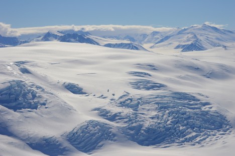
We had a spectacular flight, cutting over the end of Priestley Glacier and skirting helicopter-sized crevasses on the mountain behind our field site. Despite a bit of wind on the Nansen ice shelf, it was as calm on the Comein Glacier as it has always been for our visits. It’s such a peaceful, sheltered spot that I feel a holiday cottage wouldn’t be amiss. Perhaps too long of a commute for an average Friday afternoon, however.
Credit: NASA/Christine Dow
One of the tiltmeters (which are in black boxes) had become exposed and, because black materials absorb heat whereas white materials reflect it, had caused a bit of local melt which had trickled down the side of the box and refrozen. The upshot of this was that the entire box, battery, and straps were encased in some pretty solid ice. Fun! Commence some delicate hacking with ice axes so that we didn’t snap the wires coming out of the box. Finally having reached the interior, we nervously extracted the SD card and Ryan pulled the data off onto the computer. Success! Some excellent (and exciting) looking data showing tidal cycles. Tiltmeter two was easier because it hadn’t caused local melt of the snow so we could quickly retrieve the data. Again, some very interesting outputs. We want to thank John Leeman, an engineer from Penn State, for building us some happily working tiltmeters. Of course having disturbed the tiltmeters I had to reset them back to full level, which required sitting for 10 minutes enjoying the view while very delicately adjusting the little leveling legs.
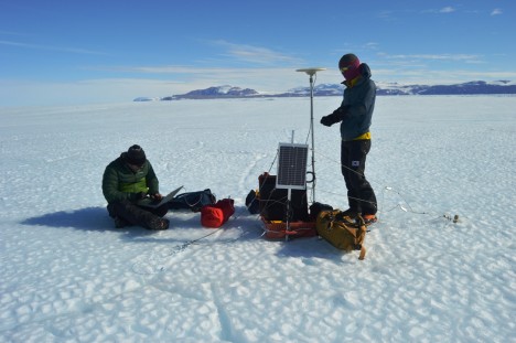
We had just enough time to collect data from one of the GPS closest to the tiltmeters. All looked well apart from our tethers, which had come loose because of melt on the surface. We had one bamboo tether and one metal peg. The metal had heated up and melted a groove in the ice as it was pulled along, whereas the bamboo had stayed where it was supposed to. We tightened the wire as much as possible but we would have to return to this site with some more bamboo later.
Credit: NASA/Christine Dow
Dinner back at base was a happy affair, having achieved success for at least three of seven of our instruments. The chefs had even made some pizza for us, which was a nice treat. The only unfortunate aspect of the day was that I had forgotten that in areas with 24 hour sunshine and highly reflective snow surfaces it is essential to put sunscreen up your nose as well as on it. Burnt nostrils are not fun, but they’re worth it for some nice data.
By Christine Dow
Credit: NASA/Christine Dow
The Nansen Ice Shelf, where we have installed our GPS, is notoriously windy. This is clear from the blue ice on the surface and complete lack of snow, which gets rapidly swept away by katabatic winds (winds driven down from the glacier towards the sea by differences in pressure induced by the cold glacier air). This means that wandering around while setting up the GPS requires spikes for your shoes or else it would be like slipping around on a scalloped ice rink. To prevent the equipment from coming loose and blowing down the ice shelf into the sea, we have a set-up where wire tethers hook our solar panel and GPS box into the ice. However, it’s always encouraging to check that the systems are holding up to the elements, so we took advantage of a helicopter flight heading in that direction to check on the field equipment. It was all still there, happily recording data.
Credit: NASA/Christine Dow
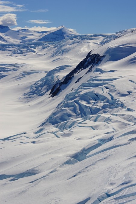
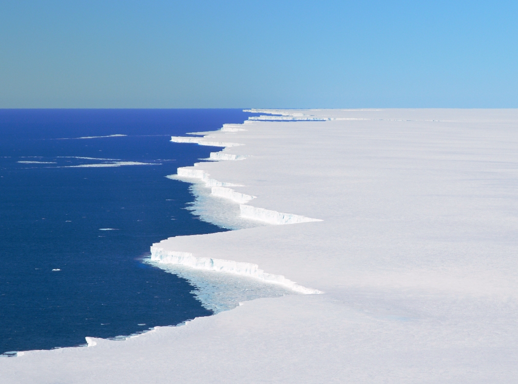
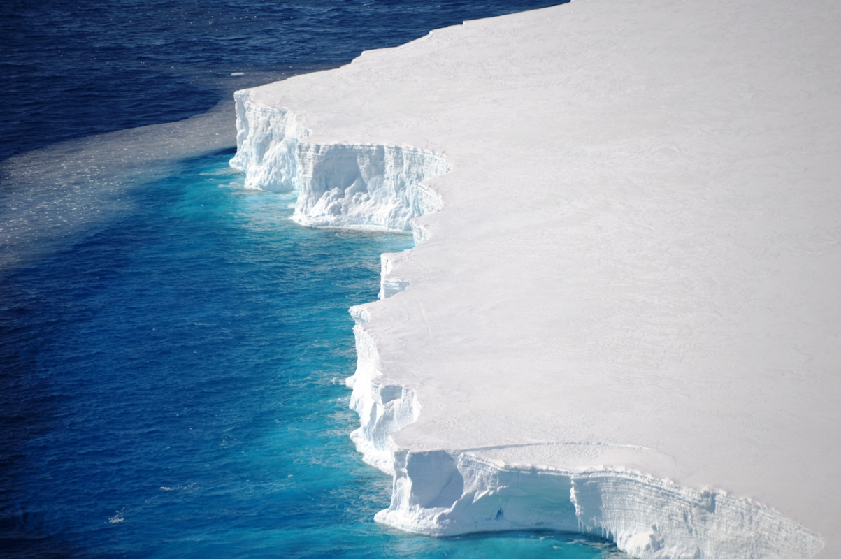
Luckily for myself and Ryan, the flight we were on was heading to the Drygalski Ice Tongue. This is a strange feature that can even be seen when looking at maps of the whole of East Antarctica. It is a floating 12 mile-wide section of ice from David glacier that sticks out 50 miles into the ocean and impacts sea ice freezing and water circulation in the bay behind it. Our approach to the ice tongue was spectacular as it headed off into the distance. At the side of the tongue, steep ice cliffs dropped into the ocean with the interaction between subsurface ice and the ocean water creating the most amazing shade of blue. We could spot groups of Adélie penguins on the remaining sections of sea ice next to the Nansen ice shelf and the Drygalski Ice Tongue.
Credit: NASA/Christine Dow
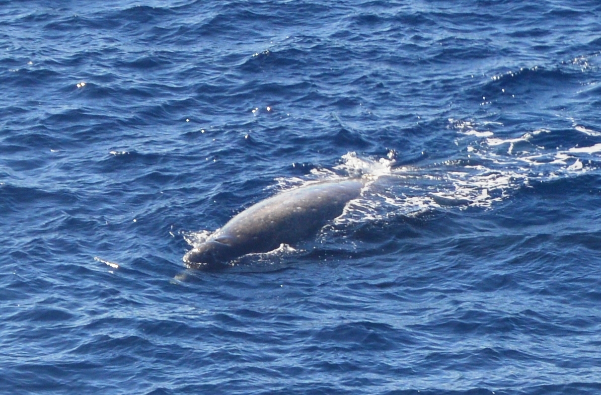
The most exciting moment was when our sharp-eyed pilot, Dom, spotted some whale spouts. We swung back around and saw four whales swimming around and breaching at the ice margin. They were Arnoux beaked whales, as we later identified, and looked nothing like any whale I have seen before – a little like very large dolphins with long pointed noses. These whales can dive for up to an hour so likely were just having a breather before heading under the ice. This was perhaps my favorite moment of the trip so far.
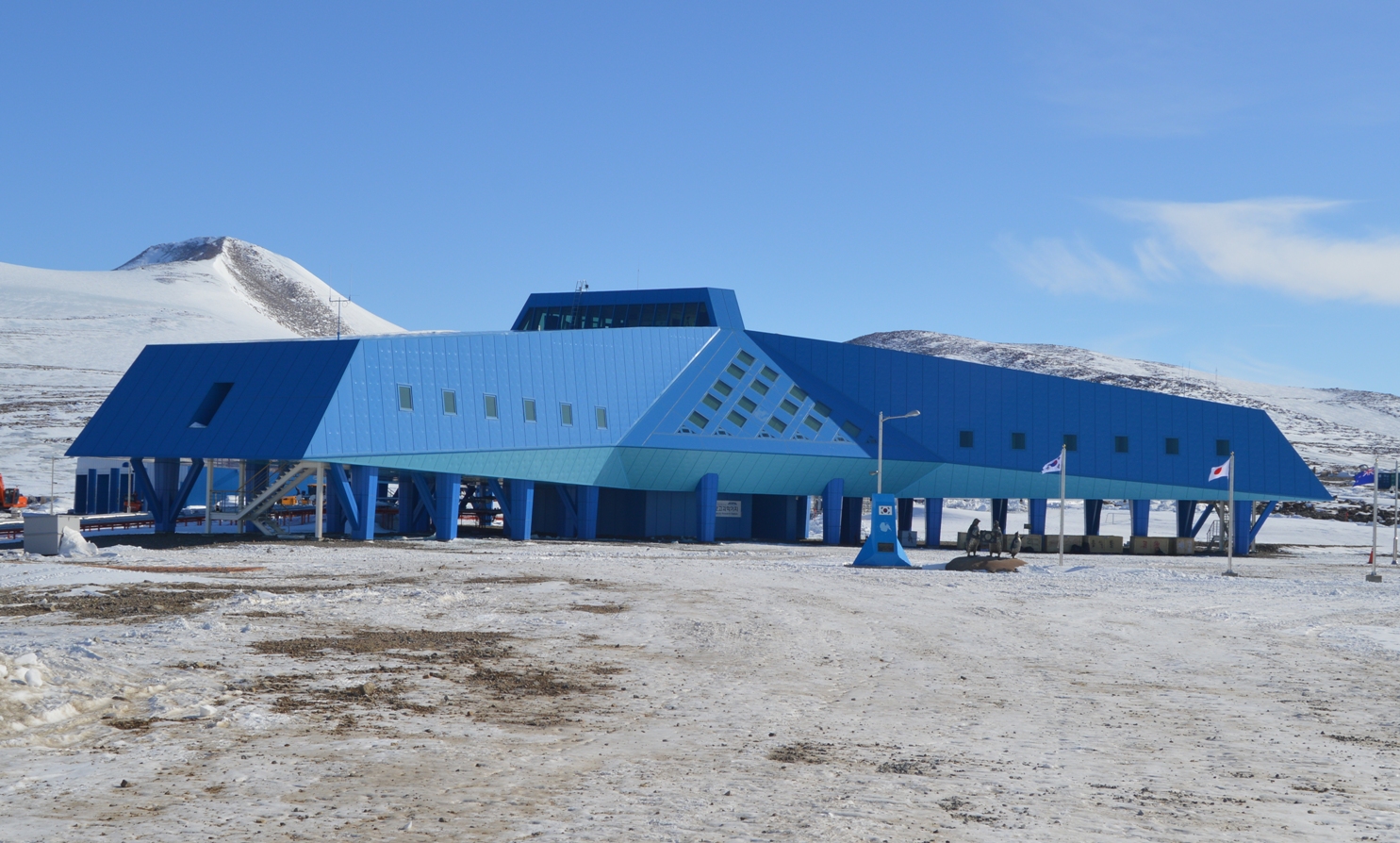
On the ice tongue we landed to check and download data from GPS stations that our Korean colleagues had installed several years before. We had a great view back across the bay towards Jang Bogo with Mt. Melbourne in the background. The second GPS site was fairly close to the front margin of the ice tongue and so Ryan and I had a geeky moment getting excited about being at the edge of one of the most bizarre ice features in the Antarctic.
It was a great day overall. All our stations were still standing, we saw wildlife, lots of ice and we were even back in time for a noodles and kimchi dinner.
By Christine Dow
Day to day life at the base station is varied primarily by timing of our field expeditions. We’ve had some very busy days getting equipment ready, deploying and checking our gear. In between, however, we are essentially operating as we would do at the office. We have set up base in the ‘Extreme Geophysics Group’ laboratory joining seven Korean scientists. Work tends to happen six days a week, with Sunday as a break (and no 7 am wake-up music!). Also on Sundays there are sometimes mini-expeditions. For example, a group of us walked a couple of miles over to Gondwana, the German base, which is semi-inhabited (two people are there at the moment keeping things ticking over). We were hoping for some “Kaffee und Kuchen” (coffee and cake) but couldn’t find anyone around. Instead we looked at rocks ejected from the nearby volcanic Mt. Melbourne, found some lichen and watched the many skuas (seabirds) flying around. We also ventured down onto the sea ice and found a nice ice slide which entertained us for a while (who said scientists couldn’t be silly).
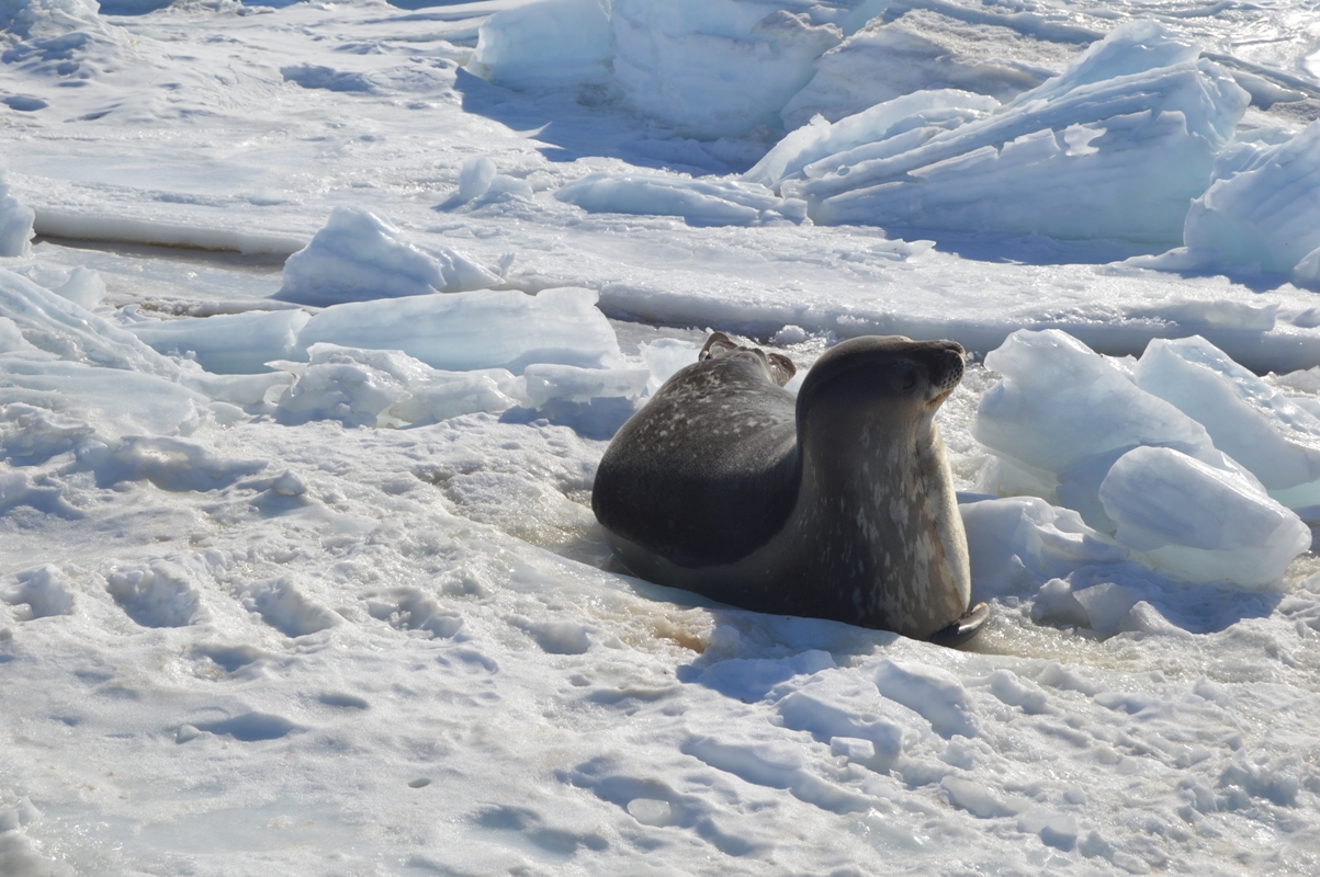
Last Sunday, Ryan and I joined a short expedition over to Mario Zucchelli, the Italian base. Recently a crack, or lead, has opened up in the sea ice so it’s no longer safe to drive the heavy Piston Bully tractors over. As an alternative, the Koreans and Italians both drove up to the crack and we exchanged passengers by hopping over the gap (it’s not really that big). There were some nearby Weddell seals hanging out near the open water, which we got a good look at. You have to be careful not to get distracted and wander into one of the seal holes which are just a bit darker than the surrounding ice – that would be a chilly surprise!
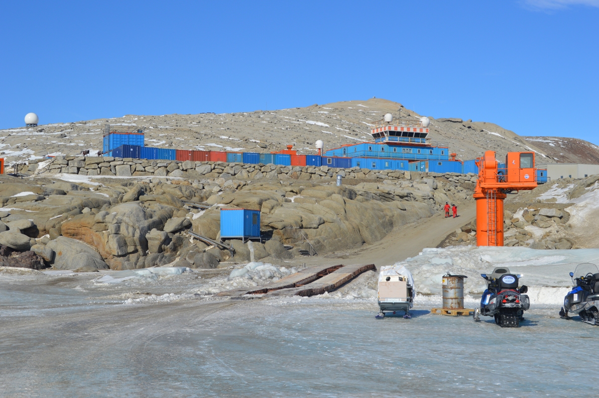
The Italian base was built 31 years ago so looks a bit more worn in than Jang Bogo but is very cosy inside. We were given a tour and fed some excellent espresso and gelato. It was really interesting to see the differences between the two bases and even the landscape. Despite being only 6 miles (10 km) apart, the rocks around Mario Zucchelli look much more weathered and eroded compared to much rougher terrain at Jang Bogo, perhaps due to the closer proximity of the volcano to the South Korean station.

At Jang Bogo, another big difference is the food and is the subject of much conversation with the Western scientists. There has been a large range of foods produced which keeps things interesting. A lot of it is a surprise since we can’t read the Korean menu, although being able to cope with spicy food is definitely an advantage (Ryan is better with this than I am). By far the best meal was Korean BBQ evening where we cooked meat and prawns on a hotplate right on the table and had a brilliant array of salad leaves (grown in house) and sundries to eat with the meat. What a meal!
