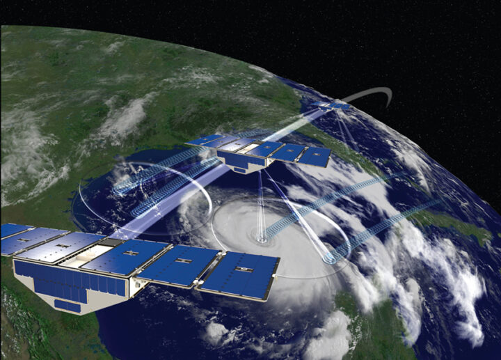
It’s been six years since the CYGNSS constellation was launched. Over that time, it has grown from a two-year mission measuring winds in major ocean storms into a mission with a broad and expanding variety of goals and objectives. They range from how ocean surface heat flux affects mesoscale convection and precipitation to how wetlands hidden under dense vegetation generate methane in the atmosphere, from how the suppression of ocean surface roughness helps track pollutant abundance in the Great Pacific Garbage Patch to how moist soil under heavy vegetation helps pinpoint locust breeding grounds in East Africa. Along with these scientific achievements, CYGNSS engineering has also demonstrated what is possible with a constellation of small, low cost satellites.
As our seventh year in orbit begins, there is both good news about the future and (possibly) bad news about the present. First the bad news. One of the eight satellites, FM06, was last contacted on 26 November 2022. Many attempts have been made since then, but without a response. There are still some last recovery commands and procedures to try, but it is possible that we have lost FM06. The other seven FMs are all healthy, functioning nominally and producing science data as usual. It is worth remembering that the spacecraft were designed for 2 years of operation on orbit and every day since then has been a welcomed gift. I am extremely grateful to the engineers and technicians at Southwest Research Institute and the University of Michigan Space Physics Research Lab who did such a great job designing and building the CYGNSS spacecraft as reliably as they did. Let’s hope the current constellation continues to operate well into the future.
And finally, the good news is the continued progress on multiple fronts with new missions that build on the CYGNSS legacy. Spire Global continues to launch new cubesats with GNSS-R capabilities of increasing complexity and sophistication. The Taiwanese space agency NSPO will be launching its TRITON GNSS-R satellite next year, and the European Space Agency will launch HydroGNSS the year after. And a new start up company, Muon Space, has licensed a next generation version of the CYGNSS instrument from U-Michigan and will launch the first of its constellation of smallsats next year.
The CYGNSS team will continue to operate its constellation, improve the quality of its science data products, and develop new products and applications for them, with the knowledge that what we develop now will continue to have a bright future with the missions yet to come. Happy Birthday, CYGNSS!
As we head into the 2018 Atlantic hurricane season, now is a good time to reflect on the accomplishments achieved by CYGNSS since its launch in December 2016. Early mission operations focused on engineering commissioning of the satellites and of the constellation as a whole. One achievement in particular is noteworthy. The satellites have no active means of propulsion, yet their relative spacing is important for achieving the required spatial and temporal sampling. The desired spacing is achieved by individually adjusting a spacecraft’s orientation and, as a result, the atmospheric drag it experiences. This technique is referred to as “differential drag”. An increase in drag will lower a satellite’s altitude, thereby changing its orbital velocity. We adjust the distance between spacecraft by adjusting their relative velocities. This is a new way of managing the spacing between a constellation of satellites, and one that can be significantly less risky and lower in cost than using traditional active propulsion. As a result, we were able to afford more satellites for the same price, which ultimately led to better, more frequent, sampling of short lived, extreme weather events like tropical cyclones.
Here is a figure, provided by CYGNSS team member Kyle Nave of ADS, illustrating the change in relative speed between two of the CYGNSS spacecraft that occurred the first time a differential drag maneuver was performed, on February 23, 2017.
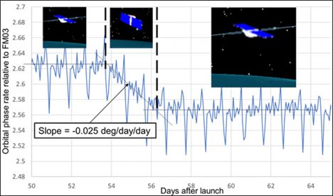
The orbital phase rate between the two spacecraft is shown before, during and after the higher of the two had its orientation changed to maximize atmospheric drag. Phase rate measures how quickly the angle between two satellites changes. By increasing the drag on the higher one, it lowers to an altitude and orbital velocity closer to the lower one, thus reducing the phase rate. This was an important first confirmation of our ability to perform the maneuver. Since then, there have been many more drag maneuvers. Five of the eight satellites are now properly positioned relative to one another at a common altitude, and the remaining three are expected to have their drag maneuvers completed later this year.
The primary science objective of the CYGNSS mission is measurement of near surface wind speed over the ocean in and near the inner core of tropical cyclones. In an earlier NASA blog, (15 Dec 2017), I reported on our measurements of Hurricane Maria made in September 2017. Since that time, we have been examining the quality of our measurements both within and away from major storms. Measurements at ocean wind speeds below 20 m/s (44 mph) were found to have an RMS uncertainty of 1.4 m/s (3 mph). Measurements of storm force winds during the 2017 Atlantic hurricane season were found to have an uncertainty of 17% of the wind speed. The analysis that produced these results is reported in Ruf et al. (2018). DOI: 10.1109/JSTARS.2018.2825948.
CYGNSS operates continuously, over both ocean and land, and the land data have been another focus of recent investigations. The quality of some of those measurements, in particular regarding its spatial resolution, has come as something of a pleasant surprise. Here is one example of CYGNSS land imagery, of the Amazon River basin in South America, provided by Dr. Clara Chew of UCAR.
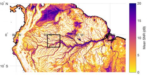
In the image, inland water bodies are prominently visible. This includes not only the major arms of the Amazon River but also its quite narrow minor tributaries. Careful examination of this and similar CYGNSS images suggests that the spatial resolution is markedly better here than it is over typical open ocean areas. The explanation lies in a transition of the electromagnetic scattering from an incoherent, rough surface regime over ocean to a largely coherent, near specular regime over inland waters. The fact that coherently scattered signals have inherently better spatial resolution is a well known phenomenon. What was unexpected is the widespread, global extent to which land surface conditions support coherent scattering. It requires the height of the surface roughness to be significantly below the wavelength of the radiowave signal, which in our case is 19 cm. This is apparently a ubiquitous property of wetland regions. It is a very fortuitous property for us, as it should enable an entirely new direction in scientific applications of CYGNSS measurements over land. NASA has recently added new investigators to the CYGNSS team specifically to study these new and exciting land applications.
A recent article summarizing these and other CYGNSS achievements, as well as some of the future applications of its measurements, is available at <www.nature.com/articles/s41598-018-27127-4>. The mission has demonstrated that smaller, more cost-efficient satellites are able to make important contributions to the advancement of science. In the months and years ahead, CYGNSS will hopefully be able to demonstrate that those advances can lead to practical scientific applications, such as extreme weather monitoring and prediction, that will benefit humankind.
CYGNSS was launched into low Earth orbit on December 15, 2016 at 08:37 EST and today is its first anniversary. The mission has had a very busy first year on orbit, transitioning from an early engineering commissioning phase into the science observing phase in time for the very active 2017 Atlantic hurricane season. The mission was supported during the hurricane season by the NOAA Airborne Operations Center (AOC), which operates a fleet of P-3 “hurricane hunter” airplanes that make reconnaissance flights into tropical storms and hurricanes to observe wind speed and other weather conditions first hand. We worked closely with AOC to coordinate many of their flight campaigns with overpasses of the storms by CYGNSS. They were able to time many of their eyewall penetrations to align closely in both time and space with our overpasses, which helps us train and evaluate our own wind speed measurements As a result, we now have dozens of coincident tracks of wind speed observations through the inner core regions of Hurricanes Harvey, Irma, Jose and Maria. The collaboration with NOAA this summer and fall has been incredibly fruitful, and I and the CYGNSS project team are very grateful for their generous support.
As the 2017 hurricane season winded down, we turned our attention to processing the coincident overpass data and characterizing and evaluating the performance of our wind speed measurements. One example is shown here. On September 24, 2017 at 18:13-18:21 UTC, the CYGNSS FM#2 spacecraft flew across Hurricane Maria.
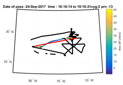
The red line in the figure shows the track of the specular reflection from transmissions by the GPS PRN#13 satellite. CYGNSS makes its wind measurements along this track. The black line in the figure shows the flight path of the P-3 hurricane hunter that day. A distinctive cloverleaf pattern can be seen that results from the plane making multiple eyewall penetrations. The colored portion of the P-3 flight path is the leg closest in time and space to the CYGNSS specular point track. The color scale represents the difference in time between the CYGNSS overpass and the P-3 observing time. With such close coincidence in time and space, we hope and expect that the two measurements of wind speed will be consistent.
The next figure shows the wind speed measured by CYGNSS (blue), measured by the P-3 airplane using its Stepped Frequency Microwave Radiometer (SFMR) wind speed sensor (red), and produced by the ECMWF and GDAS numerical weather prediction (NWP) models (black) along the CYGNSS specular point track.
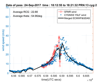
Away from the storm center at lower wind speeds, CYGNSS and NWP measurements agree well. Near the storm center, CYGNSS responds to the much higher wind speeds. In general, NWP models tend to underestimate peak winds in large storms and this is likely the case here. While NWP models generate winds everywhere, SFMR winds are only available along the portion of the satellite track where the P-3 airplane flew. In the region where coincident measurements were made, CYGNSS and SFMR winds can be seen to agree fairly well. It should be noted that the scatter present in the CYGNSS measurements can be seen to increase as the wind speed increases. This is probably a result of the decrease in GPS signal strength scattered in the specular direction when the sea surface is significantly roughened by high winds. How best to handle this characteristic of the CYGNSS wind speed retrievals will be an important topic of upcoming investigations.
Happy Birthday, CYGNSS!
p.s. and just in time for the first year anniversary of CYGNSS on orbit, new science data files using the latest (v2.0) engineering calibration and science retrieval algorithms have just been posted at the NASA PO.DAAC web site. Access the data by going to
https://podaac.jpl.nasa.gov/dataset/CYGNSS_L1_V2.0
https://podaac.jpl.nasa.gov/dataset/CYGNSS_L2_V2.0
https://podaac.jpl.nasa.gov/dataset/CYGNSS_L3_V2.0
and selecting the ‘Data Access’ tab to reach an FTP link to the data files.
Numerical weather prediction models can be run with CYGNSS data included before the satellites are even in space. This is the premise behind the Observing System Simulation Experiment, or OSSE. In an OSSE, simulated measurements from any observation platform (past, present, or future) can be assimilated into a model and their impact can then be evaluated by comparing forecasts made with and without those measurements. For an introduction to CYGNSS and how it works, please read this previous blog post.
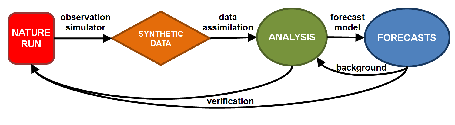
Idealized flow chart of an OSSE.
In an OSSE, the “real world” is actually high-resolution, high-quality model output from a “nature run”. That nature run is the foundation from which all observations are simulated and against which all analyses and forecasts are verified. Since the observing characteristics of instruments are known, “synthetic data” from any existing or future observation platform can be interpolated from the nature run and assigned realistic errors. If you’re living in the nature run, those synthetic data would be what your instruments would measure… including radiosondes, satellites, aircraft, buoys, and yes, even ocean surface wind speed retrievals from CYGNSS. [Note that times, dates, and events associated with the nature run are arbitrary — they do not coincide with specific events in the real world.]
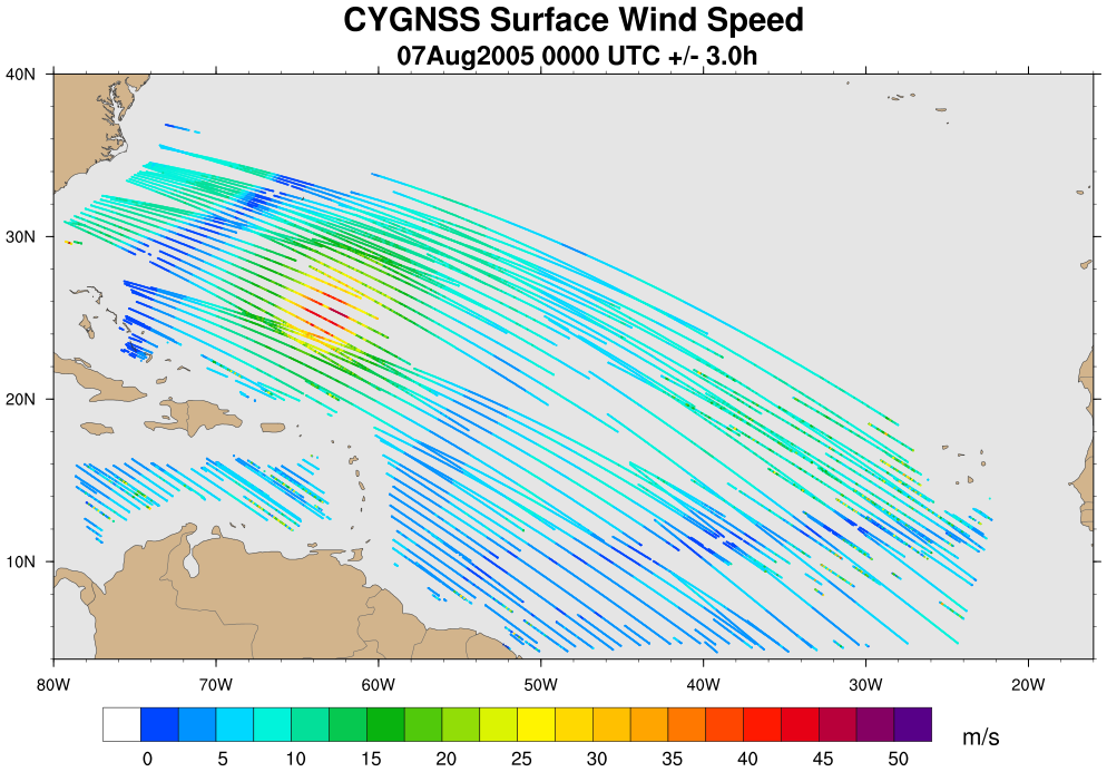
An example of synthetic CYGNSS wind speed data spanning a six hour period over the Atlantic Ocean. A hurricane can be seen north of the Lesser Antilles.
Then, the suite of observations are made available to a data assimilation (DA) system. While there are a variety of DA flavors, the basic idea is that all available observations are taken into consideration in an optimal and dynamically-consistent way to produce a best guess of the current state of the entire atmosphere. This is called the “analysis”.
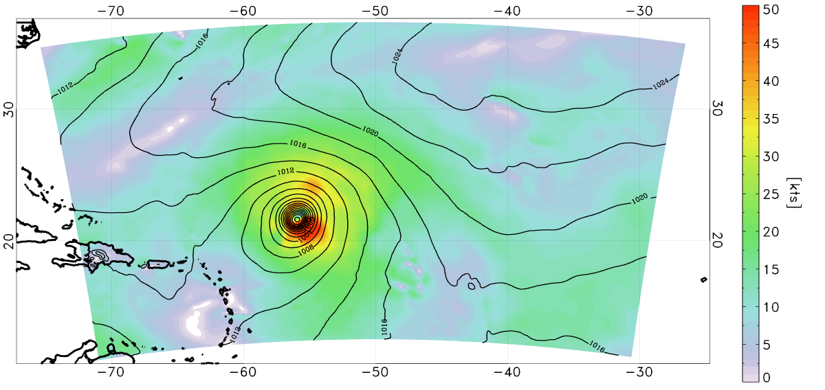
Analysis of the surface wind speed (shaded) and surface pressure (lines) on August 5 at 0000 UTC. The data assimilation method used here was a 3-D variational analysis scheme called GSI. This includes all available CYGNSS data within +/- 3 hours of the analysis time, as well as many other conventional data types.
The analysis provides the initial state for a forecast model. The forecast model, which must not be the same model used to generate the nature run, is integrated out in time. A short-term forecast (e.g. 6 hours) is used as the “background”, or first guess, for the next cycle’s analysis. Typically, the further out a forecast is run, the more it deviates from reality due to model errors, observation errors, and chaos.
The forecast model is used to produce a “control run”, which is one that includes a fixed set of observations or has a particular model configuration. Any additional data or tweaks to the DA/model system would be used to generate different runs, or experiments (“what happens if we add this”, or “what happens if we change that”). The model run is verified against the nature run by calculating errors in the analyses and forecasts — remember, the nature run is the real world in an OSSE. Output from each of the experiments can be compared to the control run to test if the errors were reduced or increased. Ideally, the addition of a new observation type such as CYGNSS improves upon the control run, but it is not always so simple in practice.
The plots below show errors in peak surface wind speed, minimum central pressure, and track for a tropical cyclone in the nature run from a control run (black line) and a single experiment with realistic CYGNSS data (red line). All of the errors from twelve forecast cycles are averaged together at the analysis time (0 hour), at 6 hours, and so on out through 120 hours. This is only an example from a single experiment, but other experiments conducted by our team include varying the DA cycling frequency, introducing “perfect” CYGNSS data interpolated directly from the nature run, adding realistic directions to the wind speeds, and assimilating higher-resolution CYGNSS data.

Errors in peak surface wind (left), minimum central pressure (middle), and track (right) for the control run (black line) and an experiment in which realistic CYGNSS data were introduced (red line). Note that lower error is ‘up’ on the y-axis on the left panel.
Based on results from a single tropical cyclone in a single nature run, simulated CYGNSS surface wind speed data do seem to have a positive impact on both analyses and short-range forecasts of tropical cyclone intensity. However, the impact on tropical cyclone track is not very noticeable, likely due to the limited influence of surface wind speeds on the storm’s steering levels.
Now we wait (im)patiently for when real data get collected and assimilated into models!
–Brian is a Senior Research Associate at the University of Miami’s Rosenstiel School of Marine and Atmospheric Science, and also blogs about hurricanes for the Washington Post.
