As we head into the 2018 Atlantic hurricane season, now is a good time to reflect on the accomplishments achieved by CYGNSS since its launch in December 2016. Early mission operations focused on engineering commissioning of the satellites and of the constellation as a whole. One achievement in particular is noteworthy. The satellites have no active means of propulsion, yet their relative spacing is important for achieving the required spatial and temporal sampling. The desired spacing is achieved by individually adjusting a spacecraft’s orientation and, as a result, the atmospheric drag it experiences. This technique is referred to as “differential drag”. An increase in drag will lower a satellite’s altitude, thereby changing its orbital velocity. We adjust the distance between spacecraft by adjusting their relative velocities. This is a new way of managing the spacing between a constellation of satellites, and one that can be significantly less risky and lower in cost than using traditional active propulsion. As a result, we were able to afford more satellites for the same price, which ultimately led to better, more frequent, sampling of short lived, extreme weather events like tropical cyclones.
Here is a figure, provided by CYGNSS team member Kyle Nave of ADS, illustrating the change in relative speed between two of the CYGNSS spacecraft that occurred the first time a differential drag maneuver was performed, on February 23, 2017.
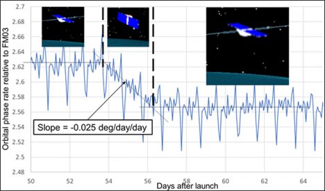
The orbital phase rate between the two spacecraft is shown before, during and after the higher of the two had its orientation changed to maximize atmospheric drag. Phase rate measures how quickly the angle between two satellites changes. By increasing the drag on the higher one, it lowers to an altitude and orbital velocity closer to the lower one, thus reducing the phase rate. This was an important first confirmation of our ability to perform the maneuver. Since then, there have been many more drag maneuvers. Five of the eight satellites are now properly positioned relative to one another at a common altitude, and the remaining three are expected to have their drag maneuvers completed later this year.
The primary science objective of the CYGNSS mission is measurement of near surface wind speed over the ocean in and near the inner core of tropical cyclones. In an earlier NASA blog, (15 Dec 2017), I reported on our measurements of Hurricane Maria made in September 2017. Since that time, we have been examining the quality of our measurements both within and away from major storms. Measurements at ocean wind speeds below 20 m/s (44 mph) were found to have an RMS uncertainty of 1.4 m/s (3 mph). Measurements of storm force winds during the 2017 Atlantic hurricane season were found to have an uncertainty of 17% of the wind speed. The analysis that produced these results is reported in Ruf et al. (2018). DOI: 10.1109/JSTARS.2018.2825948.
CYGNSS operates continuously, over both ocean and land, and the land data have been another focus of recent investigations. The quality of some of those measurements, in particular regarding its spatial resolution, has come as something of a pleasant surprise. Here is one example of CYGNSS land imagery, of the Amazon River basin in South America, provided by Dr. Clara Chew of UCAR.
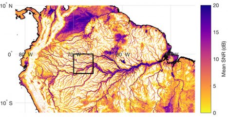
In the image, inland water bodies are prominently visible. This includes not only the major arms of the Amazon River but also its quite narrow minor tributaries. Careful examination of this and similar CYGNSS images suggests that the spatial resolution is markedly better here than it is over typical open ocean areas. The explanation lies in a transition of the electromagnetic scattering from an incoherent, rough surface regime over ocean to a largely coherent, near specular regime over inland waters. The fact that coherently scattered signals have inherently better spatial resolution is a well known phenomenon. What was unexpected is the widespread, global extent to which land surface conditions support coherent scattering. It requires the height of the surface roughness to be significantly below the wavelength of the radiowave signal, which in our case is 19 cm. This is apparently a ubiquitous property of wetland regions. It is a very fortuitous property for us, as it should enable an entirely new direction in scientific applications of CYGNSS measurements over land. NASA has recently added new investigators to the CYGNSS team specifically to study these new and exciting land applications.
A recent article summarizing these and other CYGNSS achievements, as well as some of the future applications of its measurements, is available at <www.nature.com/articles/s41598-018-27127-4>. The mission has demonstrated that smaller, more cost-efficient satellites are able to make important contributions to the advancement of science. In the months and years ahead, CYGNSS will hopefully be able to demonstrate that those advances can lead to practical scientific applications, such as extreme weather monitoring and prediction, that will benefit humankind.
CYGNSS was launched into low Earth orbit on December 15, 2016 at 08:37 EST and today is its first anniversary. The mission has had a very busy first year on orbit, transitioning from an early engineering commissioning phase into the science observing phase in time for the very active 2017 Atlantic hurricane season. The mission was supported during the hurricane season by the NOAA Airborne Operations Center (AOC), which operates a fleet of P-3 “hurricane hunter” airplanes that make reconnaissance flights into tropical storms and hurricanes to observe wind speed and other weather conditions first hand. We worked closely with AOC to coordinate many of their flight campaigns with overpasses of the storms by CYGNSS. They were able to time many of their eyewall penetrations to align closely in both time and space with our overpasses, which helps us train and evaluate our own wind speed measurements As a result, we now have dozens of coincident tracks of wind speed observations through the inner core regions of Hurricanes Harvey, Irma, Jose and Maria. The collaboration with NOAA this summer and fall has been incredibly fruitful, and I and the CYGNSS project team are very grateful for their generous support.
As the 2017 hurricane season winded down, we turned our attention to processing the coincident overpass data and characterizing and evaluating the performance of our wind speed measurements. One example is shown here. On September 24, 2017 at 18:13-18:21 UTC, the CYGNSS FM#2 spacecraft flew across Hurricane Maria.
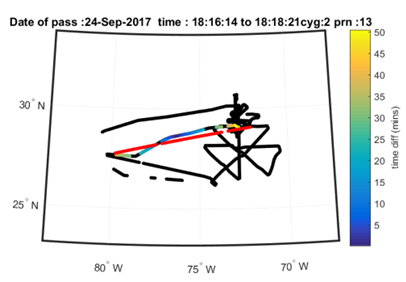
The red line in the figure shows the track of the specular reflection from transmissions by the GPS PRN#13 satellite. CYGNSS makes its wind measurements along this track. The black line in the figure shows the flight path of the P-3 hurricane hunter that day. A distinctive cloverleaf pattern can be seen that results from the plane making multiple eyewall penetrations. The colored portion of the P-3 flight path is the leg closest in time and space to the CYGNSS specular point track. The color scale represents the difference in time between the CYGNSS overpass and the P-3 observing time. With such close coincidence in time and space, we hope and expect that the two measurements of wind speed will be consistent.
The next figure shows the wind speed measured by CYGNSS (blue), measured by the P-3 airplane using its Stepped Frequency Microwave Radiometer (SFMR) wind speed sensor (red), and produced by the ECMWF and GDAS numerical weather prediction (NWP) models (black) along the CYGNSS specular point track.
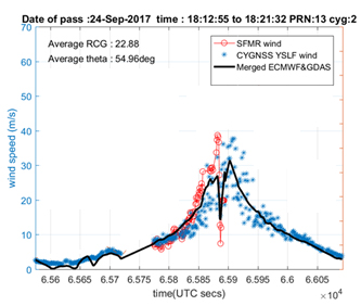
Away from the storm center at lower wind speeds, CYGNSS and NWP measurements agree well. Near the storm center, CYGNSS responds to the much higher wind speeds. In general, NWP models tend to underestimate peak winds in large storms and this is likely the case here. While NWP models generate winds everywhere, SFMR winds are only available along the portion of the satellite track where the P-3 airplane flew. In the region where coincident measurements were made, CYGNSS and SFMR winds can be seen to agree fairly well. It should be noted that the scatter present in the CYGNSS measurements can be seen to increase as the wind speed increases. This is probably a result of the decrease in GPS signal strength scattered in the specular direction when the sea surface is significantly roughened by high winds. How best to handle this characteristic of the CYGNSS wind speed retrievals will be an important topic of upcoming investigations.
Happy Birthday, CYGNSS!
p.s. and just in time for the first year anniversary of CYGNSS on orbit, new science data files using the latest (v2.0) engineering calibration and science retrieval algorithms have just been posted at the NASA PO.DAAC web site. Access the data by going to
https://podaac.jpl.nasa.gov/dataset/CYGNSS_L1_V2.0
https://podaac.jpl.nasa.gov/dataset/CYGNSS_L2_V2.0
https://podaac.jpl.nasa.gov/dataset/CYGNSS_L3_V2.0
and selecting the ‘Data Access’ tab to reach an FTP link to the data files.
The CYGNSS constellation has been operating in its science data-taking mode continuously since March 2017. The satellite hardware has been performing as designed while we make adjustments to the software on-board and on the ground so we are better able to operate smoothly and autonomously. We also spent much of the summer working on the relative spacing between the satellites, by adjusting their differential drag and, as a result, their relative orbital velocities.
An example of a typical “day in the life” for CYGNSS is shown in this video, which combines together the wind observations made by all eight spacecraft over a 24 hour period on 20 June 2017.
CYNSS wind observations (Level 3 v 1.1) made by the full constellation over a 24 hour period on 20 June 2017.
Several things are noteworthy in the video. Active storm areas appear as the regions with yellow and (especially) red wind speeds. The global coverage is seen to extend between about 38 deg north and 38 deg south latitude. If you focus on any one location within that coverage zone and note when CYGNSS measurements are made there, you can get a feel for the temporal sampling properties. In the Gulf of Mexico, for example, winds are measured during the two time interval 1300-1600 and 2000-2300 UTC. This property, that measurements are made each day during two periods of several hours each, is common to all locations within the coverage zone.
More recently, since the Atlantic hurricane season became especially active with major storms Harvey, Irma, Jose and Maria, we have focused on conducting targeted observations. This consists of predicting when we will pass over an active storm in the next several days, assembling command sequences to activate higher quality data-taking modes while over the storms, uploading those commands to the appropriate spacecraft, then scheduling additional contacts afterwards with our ground stations to downlink the higher volume of data for processing and analysis. In addition, we have been working closely with our colleagues at NOAA who operate the fleet of hurricane hunter aircraft, to coordinate their flights with our overpasses. On a number of occasions, they have been able to time the aircraft penetrations through the storm center so they coincided with CYGNSS overpasses, and to align their flight path so it paralleled the measurement track of the satellite. We are just beginning to evaluate these intercomparison data sets and intend for them to anchor our validation of high wind speed performance.
Our measurements of the major Atlantic hurricanes this season are still preliminary. The algorithms used to convert radar engineering measurements into ocean surface wind speeds have yet to be fully validated at high winds and, when they are, we will likely tweak the algorithms in order to optimize their performance. An example of CYGNSS measurements of the winds in Hurricane Harvey are shown here, taken on the morning of 25 Aug 2017. Harvey made landfall in southeast Texas that evening.
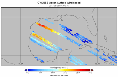
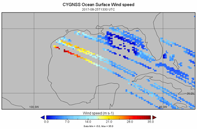
CYGNSS Level 3 gridded surface wind speed data product (v1.1). (top) at 1300-1400 and (bottom) at 1400-1500 UTC on 25 Aug 2017, prior to landfall at ~03:00 UTC on 26 Aug 2017. Hurricane Harvey is centered slightly off-shore, in the region of highest wind speeds shown in red.
CYGNSS makes measurements continuously over both ocean and land. The ocean data are used to estimate surface wind speed. The land data are sensitive to the moisture content of the soil and, in the most extreme circumstances, can be used to detect and image flood waters. This is illustrated in the following series of images of CYGNSS measurements over southeast Texas made shortly before, and then in the days after, Harvey made landfall.
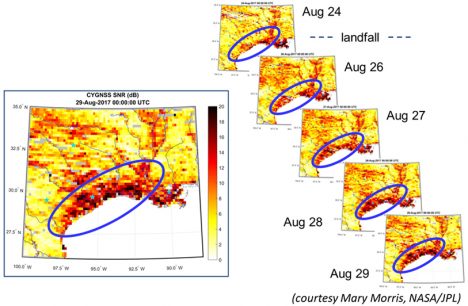
CYGNSS SNR images of southeast Texas before and after Hurricane Harvey landfall. (left) Aug 29 SNR image with coastal flooding circled. (right) Time lapse SNR images, with flooding inundation indicated by large increases in SNR.
I had the good fortune to join the crew of the NOAA P-3 “hurricane hunter” plane that flew into Harvey on 25 Aug 2017 shortly before it made landfall in Texas. We made six pairs of eyewall penetrations. The maximum surface level winds continued to grow with each successive one as we witnessed Harvey’s rapid intensification from a Cat 2 to Cat 4 hurricane. We were able to capture much of that dynamic transition, using continuous radar and radiometer remote sensing measurements plus frequent in situ measurements by dropsondes. These will be used to help calibrate and validate our measurements by CYGNSS, which have been ongoing since Harvey first started to develop earlier in the week. Following is a description of my experience that day.
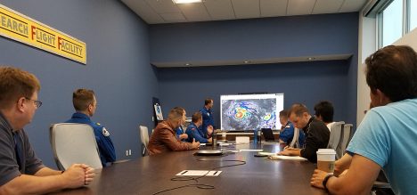
Pre-flight briefing about an hour before take-off at 10:00 EDT.
The flight out to Harvey started ominously, with a detailed safety briefing before take-off for first timers like myself about things like the difference between what to do if we have to ditch in the ocean with more than 3 minutes of warning vs. less. The hurricane hunters have been flying for decades and have never had to ditch, so this gives you some idea of how thorough and detail oriented the crew is. After the safety briefing, the flight director mustered the full crew to discuss some last minute mission logistics and concluded with this: “Harvey is currently a Cat 2 hurricane and is expected to undergo RI (rapid intensification) while we are in the air, then head for landfall tonight near a major population center. Days like today are why we are here. Now let’s go do our jobs.” We were “wheels up” 15 minutes later at 10:00 EDT.
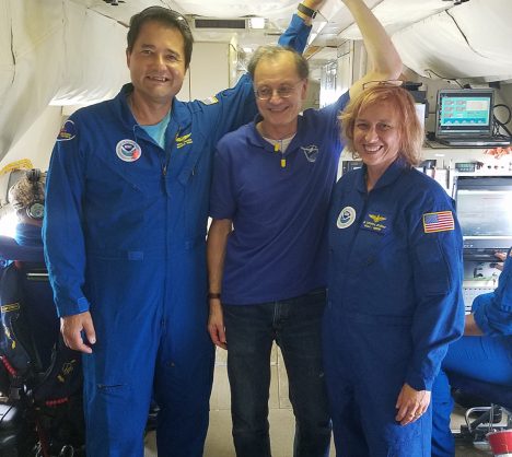
Me with two of the CYGNSS science team members, Dr. Paul Chang (left) and Dr. Zorana Jelenak (right), who were airborne mission scientists on the flight.
The two hour ferry flight from Florida across the Gulf of Mexico wasn’t much different from any commercial flight. But as we approached Harvey’s outer rain bands, things changed. Everyone strapped into their seat with four-point restraints across their chest and lap. Headsets were on and a steady chatter began between the flight director and the crew operating the various remote sensing equipment and dropsondes. A real time display from one of the radars showed the rain distribution within a 200 mile radius around us. Heavy rain spiraled out in bands from a bright circle to the south of us at the edge of the image. The plane banked to the south and headed toward that circle – the eyewall. The flight became more turbulent as we approached it. Occasionally, the bottom would drop out from under the plane and I would find myself lifted up off my seat, held down only by the straps. The flight director called it “sporty plus”. The worst of the turbulence occurred out in the spiral rain bands. Flying conditions became smoother as we approached the eyewall, but the skies grew progressively darker and, flying at 8000’ altitude and well below the freezing level, heavy rain streaked across the windows. A second real time display, from a microwave radiometer, showed the surface wind speed directly below the plane. It had been increasing steadily since we headed south into the inner core of the storm. Then we entered the eyewall. The rain became even more intense, the surface wind spiked above 51 m/s (~115 mph), and the skies darkened even more. Then, in the next minute, the interior of the plane grew suddenly brighter and the turbulence disappeared. Looking out the window, I could see the ocean below us and blue skies above. The radiometer showed that the surface wind speed had dropped below 10 m/s and the radar image drew a bright circle of intense rain all around us with nothing in the middle. We were in the eye of Harvey.
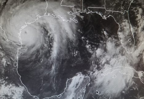
A visible image taken by the GOES satellite at 15:15 CDT as we were flying through the eye.
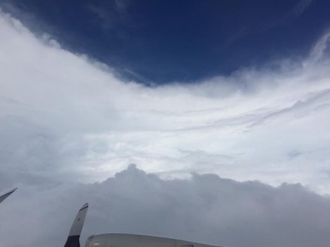
Looking out the window at 8000’ in the eye of Harvey (photo by Brad Klotz).
Over the next few hours, we conducted a total of six pairs of eyewall penetrations, each time circling to a new azimuth angle before entering the eye again in order to map out as complete an image of the storm structure as possible. With each successive penetration, the maximum winds encountered in the eyewall kept growing. We were experiencing firsthand Harvey’s rapid intensification phase as it strengthened all around us.
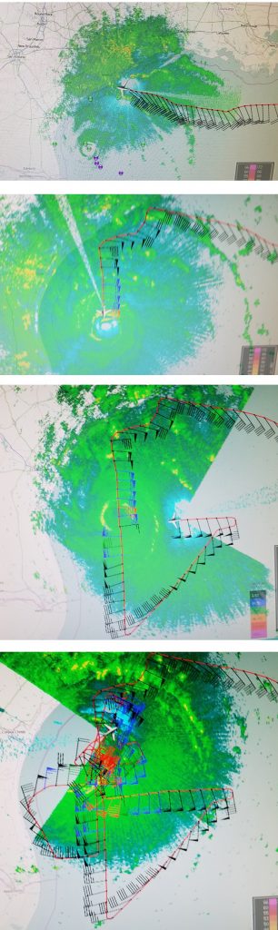
Screen captures of the flight line of the mission: (top) As we were ferrying out to the storm, when we got our first look at the eye (toward the south) with the airplane’s radar. (next) Starting our first (north-to-south) eyewall penetration. (next) Lining up for our second (east-to-west) penetration. (bottom) After our last (sixth) penetration, as we prepare to ferry back to FL.
Our measurements were radioed back to the National Hurricane Center in Miami as they were made, to be fed into their forecast models and to be forwarded to the media and emergency responders to let them know what Harvey had become and to help them prepare for what was headed toward Texas. Finally, as our fuel began to run low, we left the storm and returned back across the Gulf to our base at the NOAA Airborne Operations Center in Lakeland, FL. Minutes before landing, we received confirmation from the NHC that Harvey had been officially classified as a Cat 4 hurricane.
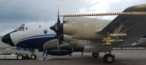
The P-3 right after we landed. Lots of hurricane remote sensors are visible on the wing and underside of the fuselage. She took very good care of us.
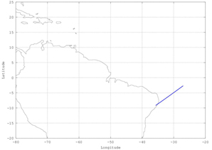
The CYGNSS constellation was launched on 15 Dec 2016 and the eight spacecraft have been going through engineering commissioning, in which each of their subsystems is tested and adjusted for best performance. One important milestone was reached on 4 Jan 2017 when we made our “first light” science measurements. This happened the first time we turned on the science radar receiver on one of the spacecraft (Flight Model #3, or FM03 for short) while pointing our science antennas down at the Earth. The receiver measures the strength of GPS signals that are reflected from the ocean surface, from which we can figure out how rough the seas are and how windy it is. FM03 was just crossing over the eastern coastline of Brazil at the time. The thick straight line pointing out into the South Atlantic from Brazil in this picture shows where FM03 was heading when we turned on the radar.
The CYGNSS radar measures four simultaneous GPS reflections that are spaced out around its sub-satellite point depending on where the GPS satellites are. Here are the first four measurements it made – our “first light” data.
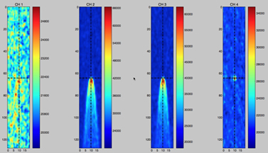
The two measurements in the middle (labeled CH2 and CH3) are good examples of what GPS reflections from the ocean should look like when everything is working properly. The bright red spot should be right in the center if the radar receiver is properly tracking the GPS transmitters, the deep blue portion above the red spot should be uniform if the receiver noise floor is nice and stable, and the tapering “horseshoe shaped” region below the red spot should be shaped just the way it is if the radar’s signal processor is working right. There are literally thousands of things that all need to be just right for images like this to be generated, so it was amazing to see them appear the first time we tried. Of course, everything was not perfect. The measurement labeled CH1 (the one on the left) shows a much noisier and fainter ocean reflection. This was as a result of the radar incorrectly looking at the ocean through a weak portion of its antenna rather than the strong part that it should be using. It was caused by a software problem that we have since fixed. The CH4 measurement on the right looks like a single hot spot without the horseshoe shaped region below it because it is a reflection from land, not ocean (possible because we were right near the Brazilian coast at the time). This is exactly what land reflections should look like, so it is not a problem.
Next, all eight of the spaceraft will have their science radar receivers turned on and we will begin to look carefully at all of the data that will begin to flow. I’ll be reporting back soon on how it looks.
